When the population standard deviation (σ) is unknown, we need to use a t-score instead of a z-score. In this case, the confidence interval formulas become:

• [latex]CL_{Lower} = \bar{x}-t \cdot \frac{s}{\sqrt{n}}[/latex]
• [latex]CL_{Upper} = \bar{x}-t \cdot \frac{s}{\sqrt{n}}[/latex]
• where [latex]E = t \cdot \frac{s}{\sqrt{n}}[/latex]

Calculating T-scores

When the population standard deviation is unknown, we must use a t-score instead of a z-score (that we used previously). We will explore what t-scores and what a t-distribution is in the next section also. For now, we will examine the 3 possible ways of calculating a t-score or the margin of error related to the t-score in Excel:

1. [latex]t = \text{T.INV.2T}(\alpha, df)[/latex]
2. [latex]t = \text{T.INV}(\frac{\alpha}{2}, df)[/latex]
3. [latex]E = \text{CONFIDENCE.T}(\alpha, {2}, s , n)[/latex]

There are two new expressions to understand in above formulas (apart from t):

• [latex]df = \text{degrees of freedom} = n - 1[/latex]
• [latex]\alpha = 1 - \text{confidence level}[/latex]

Understanding Excel’s T.INV.2T Function

When we use Excel’s T.INV.2T() function, we input the area outside of the confidence interval. This area is also called α (alpha). See figure 49.1 below to better understand this area.

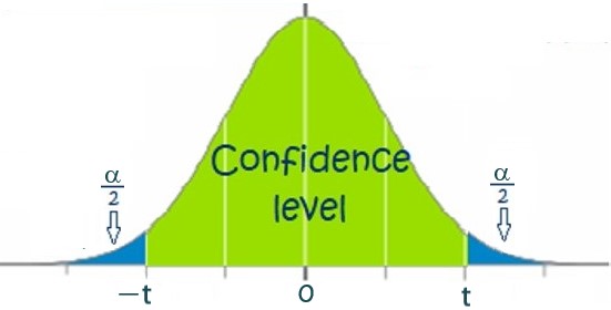
We can see from the above graph that α (alpha) makes up the area in the upper and lower tails (split between the two tails). It can be calculated using:

\[\alpha = 100\% – \text{Confidence Level} = 1 – \text{Confidence Level} \]

We can solve for [latex]t[/latex] using:

\[t = \text{T.INV.2T}(\alpha, df) \]

Finally, remember that [latex]df = n - 1[/latex]

Understanding Excel’s T.INV Function

When we use Excel’s T.INV() Function, we input the area to the left of a [latex]t[/latex]-score. The easiest is to input the area in the left tail [latex]=\frac{\alpha}{2}[/latex]. This returns the negative (−) [latex]t[/latex]-score:

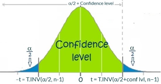
We can see from the above graph that we can solve for the negative (−) or positive [latex]t[/latex]-scores:

\[-t = \text{T.INV}(\frac{\alpha}{2}, df) = \text{T.INV}(\frac{\alpha}{2}, n-1)\]

\[t = \text{T.INV}(\frac{\alpha}{2}+\text{Conf Level}, df) = \text{T.INV}(\frac{\alpha}{2}+\text{Conf Level}, n-1)\]

Understanding Excel’s CONFIDENCE.T Function

When we use Excel’s CONFIDENCE.T() function, we input the area outside of the confidence interval (α). This function returns the Margin of Error (E):

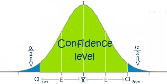
Excel’s CONFIDENCE.T() function is the quickest way to calculate the margin of error (there is no need to calculate the [latex]t[/latex]-score nor do the margin of error calculation):

[latex]E = t \cdot \frac{s}{\sqrt{n}} = \text{CONFIDENCE.T}(\alpha, {2}, s , n)[/latex]

We can easily calculate the lower and upper limits once the margin of error is known:

\[CL_{Lower} = \bar{x}-E\]

\[CL_{Upper} = \bar{x}+E\]