One Variable Hypothesis Testing
Steps to Perform a Hypothesis Test
Learning Objectives
In this section, we will:
- Introduce the six steps for hypothesis testing on either means or proportions.
- Outline the different formulae required for left, right or two-tailed tests.
With the exception of the null and alternate hypotheses and the test statistic, the steps to test if there is a difference in two population proportions is identical to the one sample hypothesis testing steps outlined in the last chapter:
- Check that the required assumptions are satisfied.
- State the Null and Alternate Hypotheses.
- Calculate the Value of the Test Statistic:
- Compute the [latex]p[/latex]-value.
- Make a Decision (to accept or reject H0).
- Draw a Conclusion (there is or is not enough evidence to conclude that an increase/decrease/change has occurred).
1. Required Assumptions
- Sample size: Is the sample size large enough to ensure that the sampling distribution is normal?
- Randomness: Are the data selected at random such that each data point is independent of the one-another. Is the sample random, representative and non-bias?
2. The Null and Alternate Hypotheses
- The Null Hypothesis (H0): There will be no observed effect for our experiment. The sample result is indeed likely from the population in question and nothing has changed. We will give examples in later sections of how exactly to define the null hypothesis.
- The Alternate Hypothesis (HA): There will be an observed effect for our experiment. The sample result not likely from the population in question and something has changed. We will give examples in later sections of how exactly to define the alternative hypothesis.
For Proportions
Let us call the original/true proportion [latex]p_{original}[/latex]. There are three possible hypothesis tests we could be performing:
- Left-tailed test: We are looking to prove that the new proportion is lower than originally stated. Ie: [latex]p < p_{original}[/latex].
- Right-tailed test: We are looking to prove that the new proportion is higher than originally stated. Ie: [latex]p > p_{original}[/latex].
- Two-tailed test: We are looking to prove that the new proportion is no longer equal to the originally stated proportion. Ie: [latex]p \neq p_{original}[/latex].
For Means
Let us call the original/true proportion [latex]\mu_{original}[/latex]. There are three possible hypothesis tests we could be performing:
- Left-tailed test: We are looking to prove that the new mean is lower than originally stated. Ie: [latex]\mu < \mu_{original}[/latex].
- Right-tailed test: We are looking to prove that the new mean is higher than originally stated. Ie: [latex]\mu > \mu_{original}[/latex].
- Two-tailed test: We are looking to prove that the new mean is no longer equal to the originally stated mean. Ie: [latex]\mu \neq \mu_{original}[/latex].
3. Test Statistic Formulae
The test statistic is a measure of how many standard errors the test statistic (x̄ or p̄) is away from the population parameter (μ or p). The formulae are:
- For Proportions: [latex]z_{test} = \frac{\bar{p}-p}{\sqrt{\frac{p(1-p)}{n}}}[/latex]
- For Means: [latex]t_{test} = \frac{\bar{x}-\mu}{\frac{s}{\sqrt{n}}}[/latex]
4. P-Value Formulae
The [latex]p[/latex]-value is the probability that the test statistic could occur, given that the null hypothesis is true (and that the sample in question originates from the original/true population). There are different formulae depending on whether we have a mean or proportion question and depending on whether we are performing a left, right or two-tailed test.
For Proportions
We will use Excel's NORM.S.DIST() function to calculate the p-values:

- Left-tailed test: [latex]p\text{-value}=\text{NORM.S.DIST}(z_{test},\text{TRUE})[/latex]
- Two-tailed test and negative z[latex]_{test}[/latex] score: [latex]p\text{-value}=2\times\text{NORM.S.DIST}(z_{test},\text{TRUE})[/latex]
- Two-tailed test and positive z[latex]_{test}[/latex] score: [latex]p\text{-value}=2\times(1-\text{NORM.S.DIST}(z_{test},\text{TRUE}))[/latex]
- Right-tailed test: [latex]p\text{-value}=1-\text{NORM.S.DIST}(z_{test},\text{TRUE})[/latex]
Note: For two-tailed tests, we double the area outside of the z[latex]_{test}[/latex] score to account for the fact that we are interested in either tail (the left or right tail). We double the area beyond the test statistic to account for this.
For Means
We can use Excel's T.DIST(), T.DIST.2T() and T.DIST.RT() functions to calculate the p-values:
- Left-tailed test: [latex]p\text{-value}=\text{T.DIST}(t_{test},n-1,\text{TRUE})[/latex]
- Two-tailed test and negative t[latex]_{test}[/latex] score: [latex]p\text{-value}=\text{T.DIST.2T}(-t_{test}, n-1)[/latex]
- Two-tailed test and positive t[latex]_{test}[/latex] score: [latex]p\text{-value}=\text{T.DIST.2T}(t_{test},n-1)[/latex]
- Right-tailed test: [latex]p\text{-value}=\text{T.DIST.RT}(t_{test},n-1)[/latex]
Note: When use T.DIST.2T, we must only input a positive t[latex]_{test}[/latex] value. For this reason, if t[latex]_{test}[/latex] is less than zero ([latex]t_{test}<0[/latex]), we add a minus (−) sign out front to 'undo' the negative value.
5. Decision Criteria
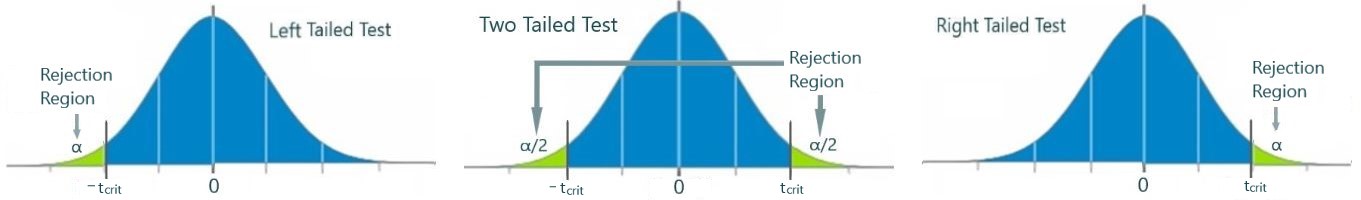
We either accept or reject the null hypothesis depending on whether the [latex]p[/latex]-value is less than the level of significance (α). We can make a diagram to visualize our decision also. If our sample result (x̄ or p̄) lands in the rejection region on our diagram, we reject H0.
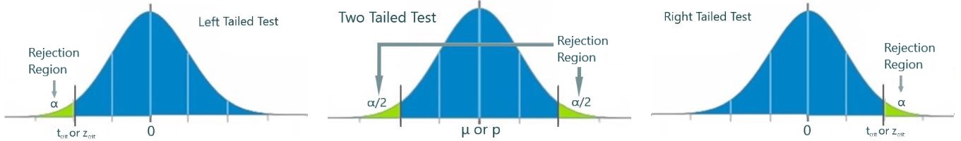
- Reject H0 if the test statistic lands in the rejection region or if the [latex]p[/latex]-value is less than (<) the level of significance (α).
- Do not reject H0 if the test statistic does not land in the rejection region or if the [latex]p[/latex]-value is more than (>) the level of significance (α).
6. Conclusions
We restate the question asked in the hypothesis test question. The following is true:
- If we reject H0: Then there is sufficient evidence to conclude what is stated in the original question (that HA is true).
- If we do not reject H0: There is not sufficient evidence to conclude what was stated in the original question (ie: there is not enough to conclude that HA is true).
