Confidence Intervals
An Introduction to Confidence Intervals
Learning Objectives
In this section, we will review
- What a confidence interval can mean
- The different types of confident intervals we can build up
- Revisit the differences between sample statistics and population parameters
- Revisit the differences between point and interval estimates
In the upcoming section, we will be building up confidence intervals:
- They can also be called "interval estimates."
- Where we are a certain "percent" confident that our population parameter lands in that interval.
- The "percent confidence" is what we will call the "confidence level."
Confidence Intervals
The figure below (Figure 47.1) shows the sampling distribution from the Normal Distributions chapter. It also shows some of the characteristics of "estimation" that we will be dealing with in this chapter. Note that the key word for an "estimation type question" is confidence. If the problem you are working on has this word in it, then you can conclude that you are dealing with estimation. Also note for the figure, that there are 3 forms of the term "confidence" that you must understand:
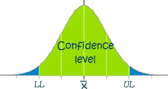
- Confidence Limits: refers to the two end points of the confidence interval as shown by "LL" and "UL" in the figure. There is a lower confidence limit and an upper confidence limit. These 2 points represent the end points of the interval.
- Confidence Interval: is the interval from the lower confidence limit to the upper confidence limit. It is not the difference between the 2 limits. In deriving the confidence interval, we will want to make sure to state that the true population parameters is between "LL" and "UL" (i.e., the 2 limits).
- Confidence Level: refers the area under the normal probability distribution (from the sampling distribution) from the lower confidence limit to the upper confidence limit.
Notes on Confidence Intervals
- There will always be some likelihood that the true population parameter will lie outside our confidence interval.
- The only way we can be absolutely certain that the truth will lie within our interval is to create an interval so wide (i.e., from infinity to infinity) that it will be useless in all practical business terms.
- For all pragmatic intervals, we must accept that there is a small chance that the true population parameter will fall outside our interval.
- This likelihood is typically kept small - less than 10% and most often under 5%.
Sample Statistic or Population Parameter?
Up to this point in time in this course, it has really not mattered if we were discussing a sample or a population. The only occurrence where it was an issue was in calculating the standard deviation. It is now important - it is impossible to solve problems without knowing if you have population parameter ([latex]\mu, \sigma, \pi[/latex]) or a sample statistic ([latex]\bar{x}[/latex], s).
Two Ways of Estimating Population Parameters
As discussed in the previous chapter, there are two ways in which we can estimate a population parameter:
- Using a Point Estimate, or
- Using an Interval Estimate.
More on Point Estimates
Recall, that a point estimate is a single value that is used to represent the population parameter. For example:
- If we are interested in determining the true average time that BCIT students spend at the pub each week (i.e., [latex]\mu[/latex]),
- What single value (i.e., a point estimate) could we use?
The answer is simple:
- Take a random and representative sample of the BCIT student population
- Calculate the sample mean [latex]\bar{x}[/latex]
- This will act as an unbiased estimator of the true average time ([latex]\mu[/latex]) that students spend at the pub each week.
As discussed in the previous chapter, even though we have some reservations concerning the accuracy of point estimates, they are still widely used in business and in our daily lives.
More on Interval Estimates
One way we can improve on estimation of the population parameters:
- Create interval estimates
- They allow us to state how certain we are that the true population parameter lies within an interval
An Example
Suppose we found from a sample of 40 students that the average time spent at the pub was 8.5 hours per week.
- We really don't know with a point estimate how far off we are from the true average time spent at the pub.
- If we had spoken with 40 different students the average time could be much more or much less.
Instead, build an interval estimate, or, confidence interval.
- Use the sample results to do so.
- This will provide a statement of how certain we are (using probability) that the true average time spent at the pub lies between [latex]x[/latex] and [latex]y[/latex] hours per week.
Three Types of Intervals
There are three types of confidence intervals we will construct in the upcoming sections:
- Confidence intervals for means where the standard deviation is known
- Confidence intervals for means where the standard deviation is unknown
- Confidence intervals for proportions
The first two sections, σ known and, σ unknown, refer to estimating the true mean of a population (μ). The third section refers to estimating the true proportion of a population (p).
