Hypothesis Testing for Two Population Proportions
Testing for Differences Examples
Learning Objectives
In this section, we will:
- perform left and two-tailed hypothesis tests for differences in proportions
- compare this test to the test in the previous chapter (see the Right-Tailed Test section below)
- recap the important formulas given in the previous section
Hypotheses
H0: [latex]p_1 = p_2[/latex], or [latex]p_1 - p_2 = 0[/latex]
HA: [latex]p_1 - p_2 < 0[/latex] (left-tailed), [latex]p_1 - p_2 > 0[/latex] (right-tailed), [latex]p_1 - p_2 \neq 0[/latex] (two-tailed)
Test Statistic
The test statistic formula is the same, regardless of what tailed test we are performing:
\[z_{test} = \frac{\bar{p_1}-\bar{p_2}}{\sqrt{\bar{p}(1-\bar{p})\left(\frac{1}{n_1}+\frac{1}{n_2}\right)}}\]
P-Values
Use Excel's NORM.S.DIST() function to calculate all p-values (see the previous section for all the formulas).
left-tailed Test (VIDEO)
Let us start by revisiting the click-through rate (CTR) Google Ads Search Network campaign example.

In the example, we will examine the following:
- The differences between the test in this section and the one proportion hypothesis test in the previous chapter.
- How this problem can be performed as both a right and left-tailed hypothesis test.
Example 61.1
Problem Setup: You and your marketing team are running an ad on Google Ad’s Search Network. You examine the Click-Through Rate before and enabling the Google’s search partners feature. Before enabling this feature, you had recorded 56 clicks on 2,946 impressions. After enabling this feature, you recorded 77 clicks-through on 3,054 impressions.
Questions: Is there sufficient evidence, at the 5% level of significance, that the click-through rate is higher when your ad can also be seen via Google's search partners?
Solutions: Click here to download the Excel solutions and click on the sections below to reveal the written solutions to each part of the above exercise.
Assumptions
- The sample size is large enough to ensure that [latex]np>5[/latex] and [latex]n(1-p)>5[/latex].
- The other conditions for before and after the feature is turned on are similar
- The are data from the samples before and after are independent of one another
- The samples are random, representative and non-bias.
Hypotheses
- H0: p1− p2 = 0
- HA: p1− p2 < 0
Rejection Region
To determine which tail we are working with (left or right), we need to think about what we are looking to prove: the click-through with the feature enabled (p2) is higher than the click-through rate without the feature enabled (p1). This gives the following:
- Click-through with feature (p2) is higher than the rate without the feature (p1)
- This gives: p2 > p1
- Moving p2 to the right side gives: 0 > p1− p2
- Flipping the inequality (read it right to left) gives: p1−p2 < 0
- If we want to prove that p1−p2 < 0, we are performing a left-tailed test.
Type of Test
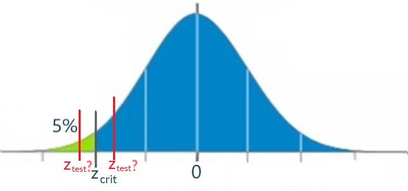
This is a left-tailed test. If p1 is much lower than p2, then their difference will be negative and the test statistic (ztest) will be low enough to be in the rejection region on the far left of the graph:
Test Statistic
First, let us calculate the sample proportions:
- [latex]x_1 = 56[/latex] and [latex]n_1 = 2946[/latex] gives [latex]\bar{p_1} = \frac{56}{2946}= 0.0190[/latex]
- [latex]x_2 = 77[/latex] and [latex]n_2 = 3054[/latex] gives [latex]\bar{p_2} = \frac{77}{3054}= 0.0252[/latex]
- [latex]\bar{p} = \frac{x_1+x_2}{n_1+n_2} = \frac{56+77}{2946+3054} = 0.02217[/latex]
We can now calculate the test statistic:
[latex]z_{test} = \frac{\bar{p_1}-\bar{p_2}}{\sqrt{\bar{p}(1-\bar{p})\left(\frac{1}{n_1}+\frac{1}{n_2}\right)}} = \frac{0.0191-0.0252}{\sqrt{0.02217(1-0.02217)\left(\frac{1}{2946}+\frac{1}{3054}\right)}} = -1.6318[/latex]
P-value
We are performing a left-tailed and use Excel's NORM.S.DIST function:
[latex]p\text{-value}=\text{NORM.S.DIST}(-1.6318, 1) = 0.0514[/latex]
Decision
Because the p-value = 0.0514 (5.14%) is greater than (>) the level of significance of 5% (0.05), we fail to reject H0.
Conclusion
Because we failed to reject H0, there is not sufficient evidence to conclude that the click-through rate is higher when the feature is turned on than when it's turned off.
RIGHT-tailed Test (Exercise)
What if, instead, we wanted to define the test as a right-tailed test. What would be different? Complete the exercise in the example below to determine the difference. In addition, let us reflect on how this example is different than the one sample proportion test from the previous chapter.
Example 61.2
Problem Setup: Let us redo the problem in Example 61.1 but solve it using a right-tailed hypothesis test.
You Try: Answer the questions in the exercise below to solve this problem:
Solutions: Click here to download the Excel solutions or click the sections below to reveal their solutions.
How One-Sample and Two-Sample Tests Are Different
In differences between Two Proportions testing (this example):
- We are testing if the two populations are different (before and after the feature is enabled).
- We are assuming that we don't know the 'true' proportion but have two different sample proportions (with and without the feature enabled) recorded.
- We use both sample proportions to come up with a 'best guess' for the population proportion, which we call the pooled sample proportion (p̄).
In One-Sample Proportion Hypothesis Testing (Example 58.1):
- We are testing the true proportion (the click-through rate) has changed from its historical value (the rate before the feature was enabled)
- We treat the historical value as our population proportion
- We compare to this amount to see if there is any difference
Setting Up the Problem as Right-Tailed
We want to prove that the rate after the feature is enabled is higher than without the feature being enabled. If we set the following to be true:
- p1 = the true click-through rate after the feature is enabled
- p2 = the true click-through rate after the feature is enabled
Then, when proving that the click-through rate is higher with the feature enabled, we get:
- HA: p1 > p2 or HA: p1 − p2 > 0
- This is a right-tailed test
The Null and Alternate Hypotheses
From the previous section, we can determine the null and alternate hypotheses:
- H0: p1 = p2 or HA: p1 − p2 = 0
- HA: p1 > p2 or HA: p1 − p2 > 0
The Test Statistic
Let us first calculate the sample proportions:
- [latex]x_1 = 77[/latex], [latex]n_1 = 3054[/latex], [latex]p_1 = \frac{77}{3054}=0.0252[/latex]
- [latex]x_2 = 56[/latex], [latex]n_2 = 2946[/latex], [latex]p_2 = \frac{56}{2946}=0.0190[/latex]
- [latex]\bar{p}=\frac{x_1+x_2}{n_1+n_2}=\frac{77+56}{3054+2946} = 0.02217[/latex]
We can now use those proportions to calculate the test statistic:
[latex]z_{test} = \frac{\bar{p_1}-\bar{p_2}}{\sqrt{\bar{p}(1-\bar{p})\left(\frac{1}{n_1}+\frac{1}{n_2}\right)}} = \frac{0.0252-0.0191}{\sqrt{0.02217(1-0.02217)\left(\frac{1}{3054}+\frac{1}{2946}\right)}} = 1.6318[/latex]
P-value
We are performing a right-tailed and use Excel's NORM.S.DIST function:
[latex]p\text{-value}=1-\text{NORM.S.DIST}(1.6318, 1) = 0.0514[/latex]
Decision
Because the p-value = 0.0514 (5.14%) is greater than (>) the level of significance of 5% (0.05), we fail to reject H0.
Conclusion
Because we failed to reject H0, there is not sufficient evidence to conclude that the click-through rate is higher when the feature is turned on than when it's turned off.
TWO-tailed Test (Video of Written Solutions)
In this example, we will perform a two-tailed hypothesis test to test if there is a difference in proportions between two populations. In this case, we will look at sentiment surrounding the LNG pipeline in British Columbia.
Example 61.3
Problem Setup: The BC Government is conducting a survey on people's sentiments toward the natural gas pipeline being built.

They have sampled two different groups - those who voted for the NDP in the previous election and those who voted for the Liberals. They found the following to be true:
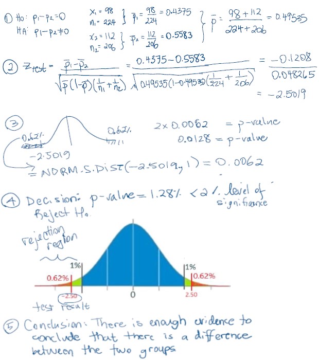
- Out of 224 NPD supporters sampled, 98 were in favor of the LNG pipeline.
- Out of 206 Liberal supporters sampled, 115 were in favor of the LNG pipeline.
Question: Is there sufficient evidence to conclude, at the 2% level of significance, that there is a difference in the proportion of people who support the pipeline between the two groups?
Solution: Click here to download the Excel solutions, or here for the PDF solutions. Finally, click below to reveal the solutions.
Click here to reveal the written solutions