Hypothesis Tests to Compare Two Population Means
Matched-Pair Differences Example
Learning Objectives
This section review the following learning objectives.
- Set up a Matched-Pair t-Test
- Use Excel’s Data Analysis Toolpak to calculate values in the test
- Draw conclusions based off of your test results
Let us first recap what types of scenarios where testing for differences in two population means uses a matched-pair test:
- One twin of sibling from one group is matched with the other twin or sibling from the second group
- One spouse from one group is matched with their spouse in the second group
- People with similar traits are matched between the two groups
- The same individuals or items are sampled before and after some change
Setting up a Matched-Pair Test
Let us look at an example of cholesterol medication. A drug company has developed a new drug to treat high cholesterol. How do they go about testing its effectiveness?
Example 63.1.1
Problem Setup: One hundred suitable individuals were selected at random. Their baseline cholesterol levels were recorded at the start of the study. They were then instructed to take a new cholesterol-reducing medication for six months. Their cholesterol levels were re-tested. Click here to download their before and after levels. The key metrics for each sample are shown in the table below:
| Statistic | Before | After |
|---|---|---|
| Mean | 181.44 | 151.54 |
| Median | 149 | 154 |
| Mode | 86 | 154 |
| Standard Deviation | 119.25 | 48.04 |
| Variance | 14219.99 | 2307.60 |
| Skewness | 2.39 | 1.53 |
| Minimum | 77 | 78 |
| Maximum | 633 | 366 |
| Count | 100 | 100 |
Question: Is there enough evidence, at the 1% level of significance to conclude that the medication reduced the individual’s cholesterol levels? Define the problem by setting up your null and alternate hypotheses for this problem.
Solution: Let us assume that there is no difference in cholesterol levels before and after taking the medication. This is what We define this as our null hypothesis (H0):
- H0: μbefore = μafter or μbefore − μafter = 0
- In other words, our hypothesized difference between the two groups equals zero.
- Later, the p-value gives a likelihood of this hypothesis being true given our sample results.
The alternative (which we hope to be left with after rejecting H0) is that cholesterol levels are lower in the individuals after six months of taking the medication. In other words:
- The average level before taking the medication is higher than the average levels after taking the medical
- HA: μbefore > μafter or μbefore − μafter > 0
If we define the ‘before’ levels as sample 1 the ‘after’ levels as sample 2, we have a right-tailed test.
Using Excel’s Data Analysis Toolpak
Let us continue with Example 63.1. In this section, we will step through how to use Excel’s Data Analysis Toolpak to calculate the required metrics for this question.
Example 63.2
Problem Setup: Continue with Example 63.1. In this example, pick the correct test within the Data Analysis Toolpak and then run this test to determine the following metrics:
- The test statistic (ttest)
- The p-value for correct tail
- The critical value (tcrit)
Solutions: Click here to download the solutions shown in the video or click to reveal the step-by-step instructions below.
Step-by-Step Solutions
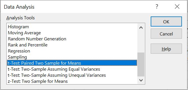
- Click on the ‘Data’ tab and select ‘Data Analysis’

- Select ‘t-test: Paired Two Sample for Means’ and click ‘OK’
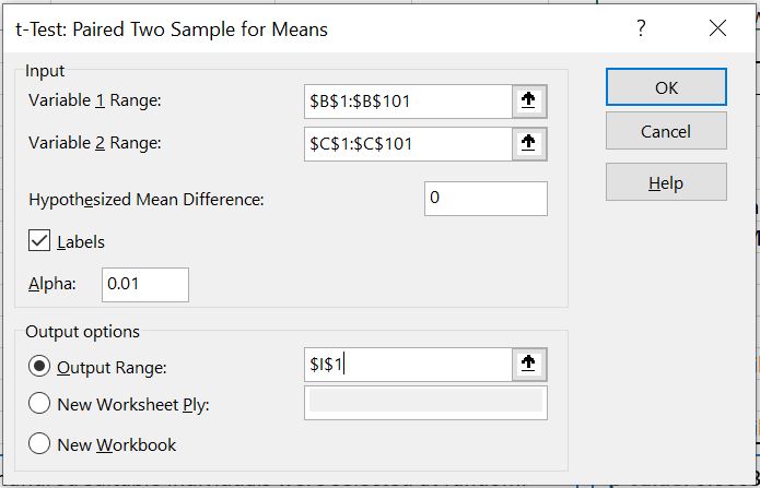
- Put the following inputs in the t-test dialogue box:
- Select the ‘Before’ column as Variable 1.
- Select the ‘After’ column as Variable 2.
- Set the Hypothesized Mean Difference to 0.
- Check off Labels.
- Enter 0.01 for Alpha (this is the level of significance)
- Select an ‘Output Range’ (either somewhere in the worksheet or a new worksheet)
- Click ‘OK’
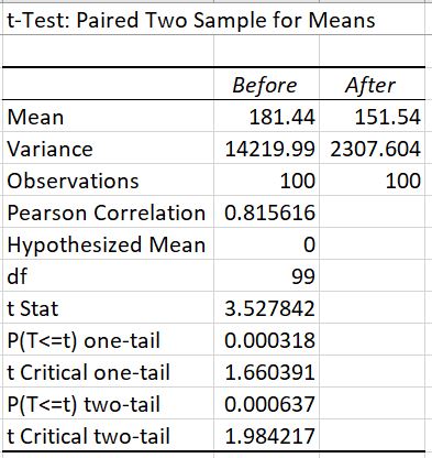
The following outputs should be given:
The Decision and Conclusion
So how do we interpret the output given by the Data Analysis Toolpak? Let us form a conclusion based off the output given in the previous section.
Example 63.3
Problem Setup: Continue with Example 63.2. Interpret the Excel output given in that example (see below).
Question: What are your decision and conclusion based on the above output?
Solutions: We are performing a right-tailed test. This is a one-tailed test. Therefore, read the P(T<=t) one-tail line to determine the p-value.
- Decision: Reject H0 at the 1% level of significance
- Reasoning: The p-value = 0.000318 is less than (<) the level of significance (0.01)
- Conclusion: There is sufficient evidence to conclude that the subjects’ average cholesterol level is lower after six months of taking the medication than before taking the medication (baseline level).
