In this section, we will step through several examples of how to perform hypothesis testing for sample means. Let us start by recapping the required formula presented in the previous section:

Hypotheses

H₀: [latex]\mu = \mu_{original}[/latex] (all tails)

H_A: [latex]\mu < \mu_{original}[/latex] (left-tailed), [latex]\mu > \mu_{original}[/latex] (right-tailed), [latex]\mu \neq \mu_{original}[/latex] (two-tailed)

Test Statistic

The test statistic formula is the same, regardless of what tailed test we are performing:

\[t_{test} = \frac{\bar{x}-\mu}{\frac{s}{\sqrt{n}}}\]

P-Values

We could use Excel’s T.DIST() function to calculate all p-values but, it is slightly easier to use different functions depending on which hypothesis test we are performing (left, right or two-tailed):

\[p_{\text{ left-tailed}}=\text{T.DIST}(t_{test},n-1,\text{TRUE})\]

\[p_{\text{ two-tailed}}=\text{T.DIST.2T}(\text{abs}(t_{test}), n-1) \]

\[p_{\text{ right-tailed}}=\text{T.DIST.RT}(t_{test},n-1)\]

Remember: When use T.DIST.2T, we must only input a positive t[latex]_{test}[/latex] value. For this reason, we can use an absolute value call ABS() to ensure that we input a positive value in the T.DIST.2T function.

Right-tailed Test (Exercise)

Let us start by working through a right-tailed hypothesis test problem for a sample with one mean.

Example 57.1

Problem Setup: Stats Canada has published a report stating that the average starting business student’s starting salary is $5,400 per month. Your college’s marketing team believes that their business diploma grads earn higher than $5,400, on average, upon graduation. A sample of 100 grads is polled and their starting salaries are reported. The average starting salary is reported at $6,500 with a standard deviation of $3,200.

Question: Is there sufficient evidence, based on the sample of 100 grads to support the marketing team’s hypothesis at a 5% level of significance?

You Try: Scroll through the questions below to solve the hypothesis test problem above.

Solutions: Click here to download the Excel solutions and click on the sections below to reveal the written solutions to each part of the above exercise.

Assumptions

• The sample size is large enough to ensure that the sampling distribution is normal.
• The are data selected at random such that each data point is independent of the one-another.
• The sample is random, representative and non-bias.

Hypotheses

• H₀: μ = $5,400
• H_A: μ > $5,400

Rejection Region

We want to prove that the mean income after graduation is higher than $5,400. For this reason, we need our sample result to be significantly higher than $5,400. The rejection region would be the upper 5% right tail. The original mean of $5,400 is what we are comparing to and is marked in the middle of the graph.

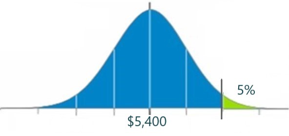
Type of Test

This is a right-tailed test. In order to prove that the mean starting salary is higher than $5,400, we will need our sample result to be far enough above the original mean of $5,400 and be, therefore, in the upper right tail (upper rejection region).

Test Statistic

[latex]\begin{align} t_{test} &= \frac{\bar{x}-\mu}{\frac{s}{\sqrt{n}}} \\ &= \frac{\$6,500-\$5,400}{\frac{\$3,200}{\sqrt{100}}} \\ &= 3.4375 \end{align}[/latex]

P-value

Because we are performing a right-tailed test on a mean, we will use Excel’s T.DIST.RT(t_test, n-1) function:

[latex]p\text{-value}=\text{T.DIST.RT}(3.4375, 99) = 0.00043[/latex]

Decision

Because the p-value = 0.00043 (0.043%) is less than (<) the level of significance of 5% (0.05), we reject H₀.

Conclusion

Because we rejected H₀, there is sufficient evidence to conclude that the college’s business diploma grads earn higher than $5,400 upon graduation.

Two-tailed Test (Exercise)

In this example, we will perform a two-tailed hypothesis test for a sample with one mean. We will return to our example of quality control for space fasteners that could be supplied to organizations and companies like NASA, SpaceX and other companies that build satellites and other machines used in space.

Example 57.2

Problem Setup: A company supplies Standard Hexagon Head Cap Screws. They perform regular quality control checks. In this case, they are performing quality control on their 5/8 inch standard hexagon head cap screws.

• They sample 100 screws.
• The mean length of the screws sampled is 0.6245 inches.
• The standard deviation of the lengths is 0.0124 inches.

Question: At the 1% level of significance, is there sufficient evidence to conclude that this batch of hexagon head cap screws are not actually 5/8 inches in length?

You Try: Scroll through the questions below to solve the hypothesis test problem above.

Solutions: Click here to download the Excel solutions and click on the sections below to reveal the written solutions to each part of the above exercise.

Assumptions

• The sample size is large enough to ensure that the sampling distribution is normal.
• The are data selected at random such that each data point is independent of the one-another.
• The sample is random, representative and non-bias.

Hypotheses

• H₀: μ = 0.625
• H_A: μ ≠ 0.625

Rejection Region

We want to prove that (or check if) the average screw length from this batch of screws is not 5/8 inches = 0.625 inches in length. When proving that the screws are not equal to 0.625 inches, we could prove this by having a batch of screws with an average length much longer or much shorter than 0.625 inches. For this reason, extreme values in either tail would prove this. This means we have a two-tailed problem:

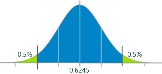
Type of Test

This is a two-tailed test, as described in the previous section. We always have a two-tailed test when the alternate hypothesis (H_A) contains a ‘not equal’ (≠) symbol.

Test Statistic

[latex]\begin{align} t_{test} &= \frac{\bar{x}-\mu}{\frac{s}{\sqrt{n}}} \\ &= \frac{0.6245-0.625}{\frac{0.0124}{\sqrt{100}}} \\ &= -0.4032 \end{align}[/latex]

P-value

Because we are performing a right-tailed test on a mean, we will use Excel’s T.DIST.RT(t_test, n-1) function:

[latex]p\text{-value}=\text{T.DIST.2T}(abs(-0.4032), 99) = 0.68765[/latex]

Decision

Because the p-value = 0.68765 (68.765%) is more than (>) the level of significance of 1% (0.01), we do not reject H₀.

Conclusion

Because we failed to reject H₀, there is not sufficient evidence to conclude that the batch of hexagon head cap screws do not have an average length of 5/8 inches.

Left-tailed Test (Exercise)

In this example, we will perform a left-tailed hypothesis test for a sample with one mean.

Example 57.3

Problem Setup: A salesman claims that his product, XYZ tires, will last at least 100,000 kilometers without failure. Your company is considering using such tires in its customized Jeeps that it manufactures however you are skeptical of the salesman’s claim. Through some laborious research you receive some information from an independent source regarding the life expectancy of XYZ tires. The independent source provides the following information on 100 randomly selected tires: the sample of tires has a mean life of 98,000 km with a standard deviation of 9,434 km.

Question: Is there sufficient evidence, at the 5% level of significance, to conclude that the salesmen’s claim regarding the life expectancy of XYZ tires is an exaggeration?

You Try: Scroll through the questions below to solve the hypothesis test problem above.

Solutions: Click here to download the Excel solutions to the above problem and click on the sections below to reveal the written solutions to each part of the above exercise.

Assumptions

• The sample size is large enough to ensure that the sampling distribution is normal.
• The are data selected at random such that each data point is independent of the one-another.
• The sample is random, representative and non-bias.

Hypotheses

• H₀: μ ≥ 100,000 or μ = 100,000 (we can always use an ‘=’ symbol for H₀)
• H_A: μ < 100,000

Rejection Region

We want to prove that the average number of kilometers the tires will last is less than 100,000 kilometers (km). If the sample of 100 tires last much less than 100,000 km, there is sufficient evidence to conclude that the real average duration of the tires is less than 100,000 km. This means we need a result in the left-tail or far below 100,000.

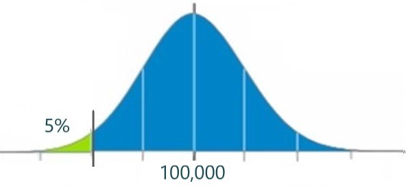
Type of Test

This is a left-tailed test. In order to prove that the mean number of kilometers that tires last is lower than 100,000 km, we will need our sample result to be far enough below the stated mean of 100,000 and be, therefore, in the lower left tail.

Test Statistic

[latex]\begin{align} t_{test} &= \frac{\bar{x}-\mu}{\frac{s}{\sqrt{n}}} \\ &= \frac{98,000-100,000}{\frac{9,434}{\sqrt{100}}} \\ &= -2.1200 \end{align}[/latex]

P-value

Because we are performing a left-tailed test on a mean, we will use Excel’s T.DIST(t_test, n-1, TRUE) function:

[latex]p\text{-value}=\text{T.DIST}(-2.12, 99, \text{TRUE}) = 0.01825[/latex]

Decision

Because the p-value = 0.01825 (1.825%) is less than (<) the level of significance of 5% (0.05), we reject H₀.

Conclusion

Because we rejected H₀, there is sufficient evidence to conclude that the salesmen’s claim regarding the life expectancy of XYZ tires is an exaggeration.