The same six steps from One Sample Hypothesis Testing still apply:

1. Check that the required assumptions are satisfied.
2. State the Null and Alternate Hypotheses.
3. Calculate the Value of the Test Statistic:
4. Compute the [latex]p[/latex]-value.
5. Make a Decision (to accept or reject H₀).
6. Draw a Conclusion (there is or is not enough evidence to conclude that one population proportion is larger/smaller/different than the other population proportion).

1. Required Assumptions

1. Sample size: Is the sample size large enough to ensure that the sampling distribution is roughly normal? For proportions, ‘large enough’ means that [latex]np > 5[/latex] and [latex]n(1-p) > 5[/latex].
2. Randomness: Are the data selected at random such that each data point is independent of the one-another. Is the sample random, representative and non-bias?

2. The Null and Alternate Hypotheses

1. The Null Hypothesis (H₀): There is no difference between the two population proportions.
   Ie: [latex]p_1 = p_2[/latex] or [latex]p_1 - p_2 = 0[/latex].
2. The Alternate Hypothesis (H_A): Either one population proportion is smaller/larger than the other (left/right-tailed) or not equal to the other:
   • Left-tailed: [latex]p_1 < p_2[/latex] or [latex]p_1 - p_2 < 0[/latex]
   • Right-tailed: [latex]p_1 > p_2[/latex] or [latex]p_1 - p_2 > 0[/latex]
   • Two-tailed: [latex]p_1 \neq p_2[/latex] or [latex]p_1 - p_2 \neq 0[/latex]

Note: Which sample is defined as the first and second samples affects which ‘tail’ (right or left) is being used. If we flip the order of the samples, we will ‘flip’ the tail (left to right or right to left).

3. THE Test Statistic FormulaE

Before calculating the test statistic, we need to perform a ‘best guess’ of the population proportion:

• We assume there is no difference between the two proportions when defining H₀
• We do not know our ‘true’/population proportion
• We combine or ‘pool’ the two sample proportions as our ‘best guess’ for the true proportion

The Pooled and Sample Proportions

Let us say that we have x₁ successes from the first sample of size n₁, and, x₂ successes from the second sample of size n_2. We can calculate the sample proportions: [latex]p_1 = \frac{x_1}{n_1}[/latex], [latex]p_2 = \frac{x_2}{n_2}[/latex]. We also use these to calculate the ‘pooled’ proportion, [latex]\bar{p}[/latex]:

\[\bar{p} = \frac{x_1+x_2}{n_1+n_2} \]

The Test Statistic (Z_test)

We can now calculate the test statistic ([latex]z_{test}[/latex]):

\[z_{test} = \frac{(\bar{p_1}-\bar{p_2})-(p_1-p_2)}{\sqrt{\bar{p}(1-\bar{p})\left(\frac{1}{n_1}+\frac{1}{n_2}\right)}} \]

This formula can be simplified by reflecting on what we assumed in our null hypothesis, H₀ (that [latex]p_1-p_2 = 0[/latex]). We replace the second term in the numerator with zero:

\[z_{test} = \frac{(\bar{p_1}-\bar{p_2})-(0)}{\sqrt{\bar{p}(1-\bar{p})\left(\frac{1}{n_1}+\frac{1}{n_2}\right)}} = \frac{\bar{p_1}-\bar{p_2}}{\sqrt{\bar{p}(1-\bar{p})\left(\frac{1}{n_1}+\frac{1}{n_2}\right)}}\]

4. The P-Value FormulaE

When testing for the differences in two proportions, the p-value equals to the probability of obtaining the sample proportion results ([latex]p_1[/latex] and [latex]p_2[/latex]) given that there is no difference in the true proportions from these two groups.

We again, use Excel’s NORM.S.DIST() function to calculate its value:

1. Left-tailed test: [latex]p\text{-value}=\text{NORM.S.DIST}(z_{test},\text{TRUE})[/latex]
2. Two-tailed test and negative z[latex]_{test}[/latex] score: [latex]p\text{-value}=2\times\text{NORM.S.DIST}(z_{test},\text{TRUE})[/latex]
3. Two-tailed test and positive z[latex]_{test}[/latex] score: [latex]p\text{-value}=2\times(1-\text{NORM.S.DIST}(z_{test},\text{TRUE}))[/latex]
4. Right-tailed test: [latex]p\text{-value}=1-\text{NORM.S.DIST}(z_{test},\text{TRUE})[/latex]

Remember: For two-tailed tests, we double the area outside of the z[latex]_{test}[/latex] score to account for the fact that we are interested in either tail (the left or right tail). We double the area beyond the test statistic to account for this.

5. Decision Criteria

We either accept or reject the null hypothesis depending on whether the [latex]p[/latex]-value is less than the level of significance (α). We can make a diagram to visualize our decision also. If our pooled proportion (p̄) lands in the rejection region on our diagram, we reject H₀.

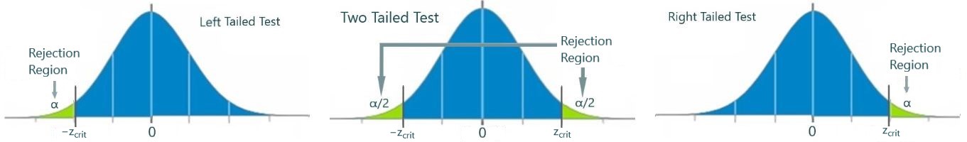
• Reject H₀ if the test statistic lands in the rejection region or if the [latex]p[/latex]-value is less than (<) the level of significance (α).
• Do not reject H₀ if the test statistic does not land in the rejection region or if the [latex]p[/latex]-value is more than (>) the level of significance (α).

6. Conclusions

We restate the question asked in the hypothesis test question. The following is true:

• If we reject H₀: Then there is sufficient evidence to conclude what is stated in the original question (that H_A is true).
• If we do not reject H₀: There is not sufficient evidence to conclude what was stated in the original question (ie: there is not enough to conclude that H_A is true).