The Central Limit Theorem

The Central Limit Theorem states that when a sample is sufficiently big:

• The distribution of the sample means (i.e., the distribution of the x ‘s) is normally distributed about the true population mean [latex]\mu[/latex].
• This distribution is called the sampling distribution (see more below).
• The standard deviation of the sample means, called the standard error, is: [latex]\sigma_{\bar{x}}=\frac{\sigma}{\sqrt{n}}[/latex]
• The z-score (standard deviations away from the mean) for sampling distributions is: [latex]z = \frac{\bar{x} -\mu}{\sigma_{\bar{x}}}[/latex]

The Sampling Distribution

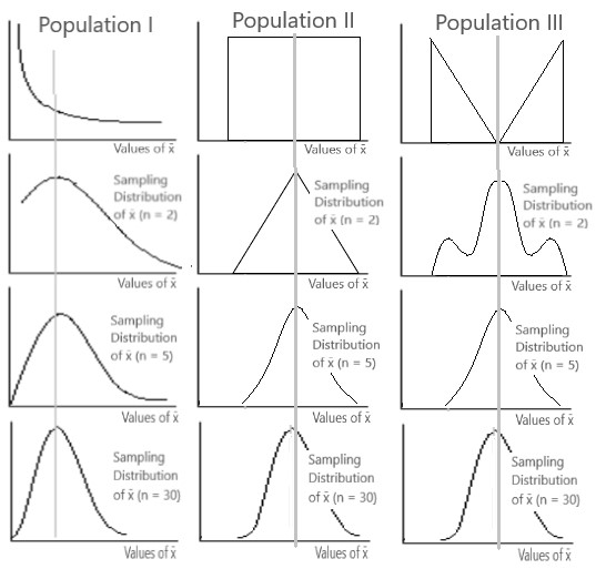
If we were to take sample after sample (of a large enough sample size) from the population, the distribution of the sample means (i.e., the distribution of all the x‘s) would form a normal distribution about the true population average. We call this distribution the sampling distribution. See Figure 45.1 below to better understand this.

Comments on Sampling Distributions

Figure 45.1 shows that in selecting simple random samples of size n from various populations:

• The sampling distribution of the sample means (the x ‘s) can be approximated by a normal probability distribution as the sample size becomes sufficiently large.
• Historically, ‘sufficiently large’ was deemed to be thirty or more. That might not be large enough in some instances.

Further Comments on Sampling Distributions

• Note that the original populations I, II and Ill have very different distributions yet the sampling distribution of the sample means (the x ‘s) are normally distributed about the true population average.
• Why this is so amazing is because this will allow us to use the normal distribution to estimate the true characteristics of the underlying population.
• The Central Limit Theorem (CLT) forms the underlying theory behind our next two topics and chapters in this text – Estimation and Hypothesis Testing

Describing the Sampling Distribution

We can describe the sampling distribution by its shape, its mean and standard deviation. Figure 45.1 shows the sampling distribution of sample means whereby its mean is defined by [latex]\mu_{\bar{x}}[/latex] and its standard deviation is defined by the standard error [latex]\sigma_{\bar{x}}[/latex].

Notation

Both the mean and the standard deviation of the sampling distribution use subscripts of [latex]\bar{x}[/latex]. As shown in Figure 45.1:

• The mean of the sampling distribution [latex]\mu_{\bar{x}}[/latex] is located about the mean of the true average of the population.
• Thus, we can say that [latex]\mu_{\bar{x}}= \mu[/latex]
• The variability of the sampling distribution is determined by the standard error [latex]\sigma_{\bar{x}}[/latex]–
• This is the standard deviation of the sample means.
• The standard error is equal to the following: [latex]\sigma_{\bar{x}}=\frac{\sigma}{\sqrt{n}}[/latex]

Effects of Increasing the Sample Size

• The sampling distribution becomes more and more bell shaped.
• The standard error, [latex]\sigma_{\bar{x}}=\frac{\sigma}{\sqrt{n}}[/latex], decreases.
• The sampling distribution gets narrower.
• In other words, our estimate of the true average gets more precise as our sample size increases.
• Or, the mean of the sampling distribution, [latex]\mu_{\bar{x}}[/latex], approaches the population mean.

Why do we not always take a large sample size?

One may ask why not take a larger sample size then? The answer to this is twofold:

1. First, as pointed out in previous sections, this would defeat the purpose of sampling to begin with as it would cost more time and money.
2. Secondly, the reduction in the standard error is not directly proportional to an increase in the sample size. The standard error decreases to a value proportional to [latex]\frac{1}{\sqrt{n}}[/latex]. Thus, in order to reduce our standard error by half, we must increase our sample size by a magnitude of 4 times its size (not 2!). Likewise, to reduce our error by two-thirds, we need to increase the sample size by an order of 9.

Sampling Distribution Parameters

We can describe the sampling distribution by its shape, mean and standard deviation (known also as the “standard error”). We know from the CLT, that the shape of the sampling distribution will be normally distributed about the true population when the sample size is 30 or more.  The mean of the sampling distribution [latex]\mu_{\bar{x}}[/latex]is equal to [latex]\mu[/latex] (the population average). The standard error (the [latex]\sigma[/latex] of the sample means) is equal to:

\[\sigma_{\bar{x}}=\frac{\sigma}{\sqrt{n}}\]

We can now update our formula for calculating the number of z-scores when dealing with a sampling distribution question:

\[z = \frac{\bar{x} -\mu}{\sigma_{\bar{x}}}\]

(we will call this “formula 10.2”)

Note that know we have both the sample mean and the population mean in the same question. Thus we need to clearly distinguish information about the sample from information about the population that is provided in the question.

In the next section we will demonstrate how the sampling distribution is used in various calculations.

Three Reasons the Normal Distribution is Important

As discussed in the previous Chapter, there are three reasons why it is important for us to study the Normal Distribution:

1. It naturally occurs in business and engineering.
2. Sometimes, it is simply easier to use to calculate other probability distributions (i.e., approximating a binomial distribution with a normal curve).
3. All sample averages, no matter what distribution they are sampled from, become normally distributed for large enough samples (according to the Central Limit Theorem).

Key Takeaways (EXERCISE)

Your Own Notes (EXERCISE)

• Are there any notes you want to take from this section? Is there anything you’d like to copy and paste below?
• These notes are for you only (they will not be stored anywhere)
• Make sure to download them at the end to use as a reference