Hypothesis Testing for Two Population Proportions

In this section, we will step through how to perform a hypothesis tests to determine if there is a difference between two population proportions.

Distribution Used

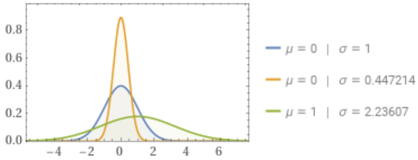
We will continued to use the Normal Distributions and z-scores.

Assumptions

In order to be able to perform the analysis in this section, the following assumptions must hold true:

• the samples are random and independent of one another
• the sample sizes and proportions from each group are large enough such that:
  • $np>5$
  • $n(1-p)>5$

Note: When the sample size and proportion are large enough, the discrete distribution approaches a normal/bell shaped curve:

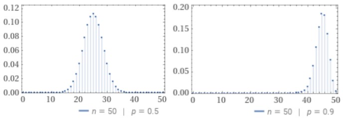
The Difference Between the Two Curves Above

For the left-most curve:

• $np=50\times 0.5=25>5$
• $n(1-p)=50\times (1-0.5)=25>5$
• the curve closely resembles a bell-shaped curve

For the right-most curve:

• $np=50\times 0.9=45>5$
• $n(1-p)=50\times (1-0.9)=5\ngtr 5$
• the curve is skewed left and therefore not bell-shaped

Note: The right-most curve is at the ‘limit’ of acceptable. If the value of $n$ was slightly larger or the value of $p$ slightly smaller (to increase the size of $1-p$), we could perform the analysis in this section on this data.