Chapter 19 Celestial Distances
19.4 The H–R Diagram and Cosmic Distances
Learning Objectives
By the end of this section, you will be able to:
- Understand how spectral types are used to estimate stellar luminosities
- Examine how these techniques are used by astronomers today
Variable stars are not the only way that we can estimate the luminosity of stars. Another way involves the H–R diagram, which shows that the intrinsic brightness of a star can be estimated if we know its spectral type.
Distances from Spectral Types
As satisfying and productive as variable stars have been for distance measurement, these stars are rare and are not found near all the objects to which we wish to measure distances. Suppose, for example, we need the distance to a star that is not varying, or to a group of stars, none of which is a variable. In this case, it turns out the H–R diagram can come to our rescue.
If we can observe the spectrum of a star, we can estimate its distance from our understanding of the H–R diagram. As discussed in Analyzing Starlight, a detailed examination of a stellar spectrum allows astronomers to classify the star into one of the spectral types indicating surface temperature. (The types are O, B, A, F, G, K, M, L, T, and Y; each of these can be divided into numbered subgroups.) In general, however, the spectral type alone is not enough to allow us to estimate luminosity. Look again at [link]. A G2 star could be a main-sequence star with a luminosity of 1 LSun, or it could be a giant with a luminosity of 100 LSun, or even a supergiant with a still higher luminosity.
We can learn more from a star’s spectrum, however, than just its temperature. Remember, for example, that we can detect pressure differences in stars from the details of the spectrum. This knowledge is very useful because giant stars are larger (and have lower pressures) than main-sequence stars, and supergiants are still larger than giants. If we look in detail at the spectrum of a star, we can determine whether it is a main-sequence star, a giant, or a supergiant.
Suppose, to start with the simplest example, that the spectrum, color, and other properties of a distant G2 star match those of the Sun exactly. It is then reasonable to conclude that this distant star is likely to be a main-sequence star just like the Sun and to have the same luminosity as the Sun. But if there are subtle differences between the solar spectrum and the spectrum of the distant star, then the distant star may be a giant or even a supergiant.
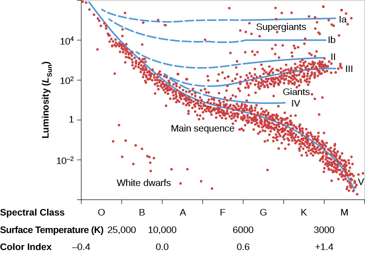
The most widely used system of star classification divides stars of a given spectral class into six categories called luminosity classes. These luminosity classes are denoted by Roman numbers as follows:
- Ia: Brightest supergiants
- Ib: Less luminous supergiants
- II: Bright giants
- III: Giants
- IV: Subgiants (intermediate between giants and main-sequence stars)
- V: Main-sequence stars
The full spectral specification of a star includes its luminosity class. For example, a main-sequence star with spectral class F3 is written as F3 V. The specification for an M2 giant is M2 III. [link] illustrates the approximate position of stars of various luminosity classes on the H–R diagram. The dashed portions of the lines represent regions with very few or no stars.
With both its spectral and luminosity classes known, a star’s position on the H–R diagram is uniquely determined. Since the diagram plots luminosity versus temperature, this means we can now read off the star’s luminosity (once its spectrum has helped us place it on the diagram). As before, if we know how luminous the star really is and see how dim it looks, the difference allows us to calculate its distance. (For historical reasons, astronomers sometimes call this method of distance determination spectroscopic parallax, even though the method has nothing to do with parallax.)
The H–R diagram method allows astronomers to estimate distances to nearby stars, as well as some of the most distant stars in our Galaxy, but it is anchored by measurements of parallax. The distances measured using parallax are the gold standard for distances: they rely on no assumptions, only geometry. Once astronomers take a spectrum of a nearby star for which we also know the parallax, we know the luminosity that corresponds to that spectral type. Nearby stars thus serve as benchmarks for more distant stars because we can assume that two stars with identical spectra have the same intrinsic luminosity.
A Few Words about the Real World
Introductory textbooks such as ours work hard to present the material in a straightforward and simplified way. In doing so, we sometimes do our students a disservice by making scientific techniques seem too clean and painless. In the real world, the techniques we have just described turn out to be messy and difficult, and often give astronomers headaches that last long into the day.
For example, the relationships we have described such as the period-luminosity relation for certain variable stars aren’t exactly straight lines on a graph. The points representing many stars scatter widely when plotted, and thus, the distances derived from them also have a certain built-in scatter or uncertainty.
The distances we measure with the methods we have discussed are therefore only accurate to within a certain percentage of error—sometimes 10%, sometimes 25%, sometimes as much as 50% or more. A 25% error for a star estimated to be 10,000 light-years away means it could be anywhere from 7500 to 12,500 light-years away. This would be an unacceptable uncertainty if you were loading fuel into a spaceship for a trip to the star, but it is not a bad first figure to work with if you are an astronomer stuck on planet Earth.
Nor is the construction of H–R diagrams as easy as you might think at first. To make a good diagram, one needs to measure the characteristics and distances of many stars, which can be a time-consuming task. Since our own solar neighborhood is already well mapped, the stars astronomers most want to study to advance our knowledge are likely to be far away and faint. It may take hours of observing to obtain a single spectrum. Observers may have to spend many nights at the telescope (and many days back home working with their data) before they get their distance measurement. Fortunately, this is changing because surveys like Gaia will study billions of stars, producing public datasets that all astronomers can use.
Despite these difficulties, the tools we have been discussing allow us to measure a remarkable range of distances—parallaxes for the nearest stars, RR Lyrae variable stars; the H–R diagram for clusters of stars in our own and nearby galaxies; and cepheids out to distances of 60 million light-years. [link] describes the distance limits and overlap of each method.
Each technique described in this chapter builds on at least one other method, forming what many call the cosmic distance ladder. Parallaxes are the foundation of all stellar distance estimates, spectroscopic methods use nearby stars to calibrate their H–R diagrams, and RR Lyrae and cepheid distance estimates are grounded in H–R diagram distance estimates (and even in a parallax measurement to a nearby cepheid, Delta Cephei).
This chain of methods allows astronomers to push the limits when looking for even more distant stars. Recent work, for example, has used RR Lyrae stars to identify dim companion galaxies to our own Milky Way out at distances of 300,000 light-years. The H–R diagram method was recently used to identify the two most distant stars in the Galaxy: red giant stars way out in the halo of the Milky Way with distances of almost 1 million light-years.
We can combine the distances we find for stars with measurements of their composition, luminosity, and temperature—made with the techniques described in Analyzing Starlight and The Stars: A Celestial Census. Together, these make up the arsenal of information we need to trace the evolution of stars from birth to death, the subject to which we turn in the chapters that follow.
| Distance Range of Celestial Measurement Methods | |
|---|---|
| Method | Distance Range |
| Trigonometric parallax | 4–30,000 light-years when the Gaia mission is complete |
| RR Lyrae stars | Out to 300,000 light-years |
| H–R diagram and spectroscopic distances | Out to 1,200,000 light-years |
| Cepheid stars | Out to 60,000,000 light-years |
Key Concepts and Summary
Stars with identical temperatures but different pressures (and diameters) have somewhat different spectra. Spectral classification can therefore be used to estimate the luminosity class of a star as well as its temperature. As a result, a spectrum can allow us to pinpoint where the star is located on an H–R diagram and establish its luminosity. This, with the star’s apparent brightness, again yields its distance. The various distance methods can be used to check one against another and thus make a kind of distance ladder which allows us to find even larger distances.
For Further Exploration
Articles
Adams, A. “The Triumph of Hipparcos.” Astronomy (December 1997): 60. Brief introduction.
Dambeck, T. “Gaia’s Mission to the Milky Way.” Sky & Telescope (March 2008): 36–39. An introduction to the mission to measure distances and positions of stars with unprecedented accuracy.
Hirshfeld, A. “The Absolute Magnitude of Stars.” Sky & Telescope (September 1994): 35. Good review of how we measure luminosity, with charts.
Hirshfeld, A. “The Race to Measure the Cosmos.” Sky & Telescope (November 2001): 38. On parallax.
Trefil, J. Puzzling Out Parallax.” Astronomy (September 1998): 46. On the concept and history of parallax.
Turon, C. “Measuring the Universe.” Sky & Telescope (July 1997): 28. On the Hipparcos mission and its results.
Zimmerman, R. “Polaris: The Code-Blue Star.” Astronomy (March 1995): 45. On the famous cepheid variable and how it is changing.
Websites
ABCs of Distance: http://www.astro.ucla.edu/~wright/distance.htm. Astronomer Ned Wright (UCLA) gives a concise primer on many different methods of obtaining distances. This site is at a higher level than our textbook, but is an excellent review for those with some background in astronomy.
American Association of Variable Star Observers (AAVSO): https://www.aavso.org/. This organization of amateur astronomers helps to keep track of variable stars; its site has some background material, observing instructions, and links.
Friedrich Wilhelm Bessel: http://messier.seds.org/xtra/Bios/bessel.html. A brief site about the first person to detect stellar parallax, with references and links.
Gaia: http://sci.esa.int/gaia/. News from the Gaia mission, including images and a blog of the latest findings.
Hipparchos: http://sci.esa.int/hipparcos/. Background, results, catalogs of data, and educational resources from the Hipparchos mission to observe parallaxes from space. Some sections are technical, but others are accessible to students.
John Goodricke: The Deaf Astronomer: http://www.bbc.com/news/magazine-20725639. A biographical article from the BBC.
Women in Astronomy: http://www.astrosociety.org/education/astronomy-resource-guides/women-in-astronomy-an-introductory-resource-guide/. More about Henrietta Leavitt’s and other women’s contributions to astronomy and the obstacles they faced.
Videos
Gaia’s Mission: Solving the Celestial Puzzle: https://www.youtube.com/watch?v=oGri4YNggoc. Describes the Gaia mission and what scientists hope to learn, from Cambridge University (19:58).
Hipparcos: Route Map to the Stars: https://www.youtube.com/watch?v=4d8a75fs7KI. This ESA video describes the mission to measure parallax and its results (14:32)
How Big Is the Universe: https://www.youtube.com/watch?v=K_xZuopg4Sk. Astronomer Pete Edwards from the British Institute of Physics discusses the size of the universe and gives a step-by-step introduction to the concepts of distances (6:22)
Search for Miss Leavitt: http://perimeterinstitute.ca/videos/search-miss-leavitt., Video of talk by George Johnson on his search for Miss Leavitt (55:09).
Women in Astronomy: http://www.youtube.com/watch?v=5vMR7su4fi8. Emily Rice (CUNY) gives a talk on the contributions of women to astronomy, with many historical and contemporary examples, and an analysis of modern trends (52:54).
Glossary
- luminosity class
- a classification of a star according to its luminosity within a given spectral class; our Sun, a G2V star, has luminosity class V, for example
