5 Decision Trees and split points
Making a decision on split points:
We are going to look at a very small example of a decision tree, and then expand a bit.
Here is our 3 item, two variable problem. We are trying to predict whether a customer purchased a new financial product, based solely on their income:
| ID | Income | Purchase |
| 1 | $12,000 | 0 (NO) |
| 2 | $15,000 | 0 (NO) |
| 3 | $25,000 | 1 (YES) |
Our Tree will look like this:
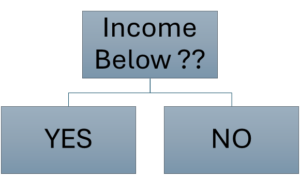
What we have to do is calculate the split point: what should be our [latex]??[/latex] in the diagram.
What we do is sort all of our data in order by income. Our candidate split points are halfway between each consecutive pair.
Here we have:
- [latex]\$13,500 = \frac{\$12,000 + \$15,000}{2}[/latex]
- [latex]\$20,000 = \frac{\$15,000 + \$25,000}{2}[/latex]
For each of these, we will count the number of 0 and 1 in each tree, and try to pick the "best" one:
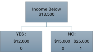
Now we calculate the probabilities of each outcome:
- [latex]P(0 | \leq \$13,500) = 1[/latex]
- [latex]P(1 | \leq \$13,500) = 0[/latex]
- [latex]P(0 | > \$13,500) = 0.5[/latex]
- [latex]P(0 | \leq \$13,500) = 0.5[/latex]
We will analyze this properly soon, but let's redo this analysis for our second candidate split point:
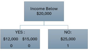
This is called a "Pure Split Point" - that is, each box has either all 0 or all 1. Our probabilities are:
- [latex]P(0 | \leq \$20,000) = 1[/latex]
- [latex]P(1 | \leq \$20,000) = 0[/latex]
- [latex]P(0 | >\$20,000) = 0[/latex]
- [latex]P(0 | > \$20,000) = 1[/latex]
This seems like a better choice! But let's quantify this:
There are three main methods of choosing the best split point, and unsurprisingly they all involve statistical measures of dispersion:
- Gini (named after a person, not an acronym!)
- Entropy
- [latex]\chi^2[/latex] measure of independence
GINI
In the Gini method, we find the Gini index for each split point, and then compare. The Gini index is a type of weighted average of the probabiliteis that we calculated above: Here, I'm going to use the word "boxes" to describe each of the end points: being less than or greater than the split point. In our simple example we have two boxes. I will use classes to describe the outcomes that are possible: 0 or 1 in our case. It's easier to look at classification that uses only 2 categories or classes, but we can extend to more classes. We will also use [latex]N[/latex] as the total number of data points. Here it is 3!
We calculate this via the equation:
\[ GINI_{split} =\Sigma_{boxes} \left[ \frac{\text{# of points in the box}}{N} \cdot Gini_{box}\right] \]
where
\[Gini_{box} =1 - \Sigma_{classes} \left( \frac{\text{number of 0 or 1 in box}}{\text{# of points in the box}}\right)^2\]
This is easier calculate than to understand the math!
Recall the chart:
We will calculate the Gini number for each part:
[latex]\begin{align*} Gini_{<13,500} &= 1 - \left[ \left(\frac{ \text{# of 0 < 13,500}} {\text{# < 13,500}} \right)^2 +\left(\frac {\text{# of 1< 13,500}} {\text{# < 13,500}}\right)^2 \right]\\ &=1- \left[ \left( \frac{1}{1}\right)^2+ \left(\frac{0}{1}\right)^2 \right]\\ & = 1 - \left[ 1 + 0 \right]\\ & = 0\end{align*}[/latex] and: [latex]\begin{align*} Gini_{>13,500} &= 1 - \left[ \left(\frac{ \text{# of 0 > 13,500}} {\text{# > 13,500}} \right)^2 +\left(\frac {\text{# of 1> 13,500}} {\text{# > 13,500}}\right)^2 \right]\\ &=1- \left[ \left( \frac{1}{2}\right)^2+ \left(\frac{1}{2}\right)^2 \right]\\ & = 1 - \left[ \frac{1}{4}+\frac{1}{4} \right]\\ & =\frac{1}{2} \end{align*}[/latex]
0 is the lowest a Gini Index can be, we call this a pure, and 0.5 is the worst case scenario.
The Index is given by:
\[ Gini_{13,500} = \left( \frac{\text{# < 13,500}}{Total}\right) \cdot Gini_{< 13,500}+ \left( \frac{\text{# >13,500}}{Total}\right) \cdot Gini_{>13,500}\]
Or:
\[Gini_{13,500} = \frac{1}{3}\cdot 0 + \frac{2}{3}\cdot \frac{1}{2} = \frac{1}{3}\]
Now we have the fun of repeating for our second split point, $20,000. This will be easier, as we do have a pure split -
\[Gini_{<20,000} = 1 -\left[\left( \frac{2}{2}\right)^2 +\left( \frac{0}{2}\right)^2 \right] = 1-1=0\]
and
\[Gini_{>20,000} = 1 -\left[\left( \frac{0}{1}\right)^2 +\left( \frac{1}{1}\right)^2 \right] = 1-1=0\]
Which gives us:
\[Gini_{20,000} = \frac{1}{3}\cdot 0 + \frac{2}{3}\cdot 0 = 0\]
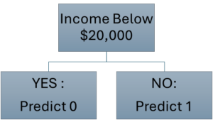
Hence, when we minimize the Gini Index, we choose $20,000 as a split point, and our algorithm now looks like this:
Of course, doing this by hand is time consuming! We really should be using a computer, if we had more than three points.
Entropy
Calculating these by hand is not a fun task, but we briefly look at a different measure, Entropy, which we are again trying to minimize.
\[Entropy_{box} = -\frac{\text{# in class}}{N} \Sigma \frac{\text{#}}{N} \cdot ln \left(\frac{\text{#}}{N}\right)\]
continue later Amy!
Decisions / hyperparameters
- Should we look at all features? Or just choose one randomly
- How many classes at each split point?
- How deep do we want the tree?
