17 What is a Vector?
Vectors
Updated Feb 2024
A vector is something which has magnitude or length and direction. It is used to describe a variety of things. We can also view a vector as an ordered n-tuple, ie, [latex](a, b, c)[/latex], or as a set of directions.
Vectors in two dimensions
In two dimensions, a vector is an ordered pair of real numbers, [latex](a,b)[/latex] or [latex]\binom{a}{b}[/latex] (expressed vertically. We use“arrow” notation to show that this has direction - as opposed to being a point. When we draw this, it has an arrow:
\[\vec{v} = \binom{1}{2}, \,\, \vec{w} = \binom{3}{1}\]
## This is a Python cell; see how we create vectors:

## We need a library, NumPy has the best math-y stuff

import numpy as np

## Define a Vector

## note that I've used 2 sets of brackets: the square ones define a list INSIDE of the function

v = np.array([1,2])

w = np.array([3,1])

print("v = ", v, " and w = ", w)
v = [1 2] and w = [3 1]Visualizing:
Usually vectors look like arrows coming out from [latex](0,0)[/latex]
## Don't worry a lot about graphing, but know that matplotlib is a pretty good tool, and lets us plot our math stuff nicely
## matplotlib also makes stats visualizations!

## Why plt?  I dunno... tradition
import matplotlib.pyplot as plt


# Creating plot
## Tells Python to dray a blue arrow from (0,0) to (1,2)
plt.quiver(0, 0, v[0], v[1], color='b', units='xy', scale=1)


## and the red line is w
plt.quiver(0, 0, w[0], w[1], color='r', units='xy', scale=1)

plt.axis('equal')
plt.title('Vectors on a Plane')

plt.xticks(range(-1,5))
plt.yticks(range(-1,5))


# Show plot with grid
plt.grid()
plt.show() 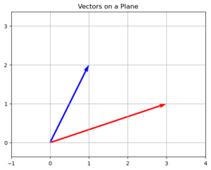
But they don’t need to start at [latex](0,0)[/latex]! Think of them as a set of instructions, saying “from any begining point, go [latex]a[/latex] steps to the right, and [latex]b[/latex] steps up.
In this plot, I have the second (red) vector start where the first one ends.
In the next plot, the blue vector is repeated a bunch of times….
# Creating plot
## Tells Python to dray a blue arrow from (0,0) to (1,2)
plt.quiver(0, 0, v[0], v[1], color='b', units='xy', scale=1)

#plt.quiver(X, Y, 1,2, color='g', units='xy', scale= 1)


## and the red line starts where the blue one ends.
plt.quiver(v[0], v[1], w[0], w[1], color='r', units='xy', scale=1)

plt.axis('equal')
plt.title('Vectors can start anywhere')

plt.xticks(range(-1,5))
plt.yticks(range(-1,5))


# Show plot with grid
plt.grid()
plt.show() 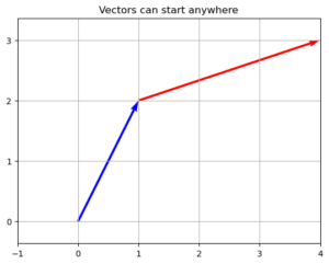
# Creating plot

 ## Tells Python to dray a blue arrow from (0,0) to (1,2)

plt.quiver([0,1,3], [0,-1,2], [v[0],v[0],v[0]], [v[1], v[1], v[1]], color='b', units='xy', scale=1)


plt.axis('equal')

plt.title('Vectors can start anywhere') plt.yticks(range(-10,10))plt.grid()
plt.show()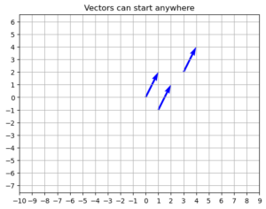
Other Vector Spaces
We can put these vectors anywhere - in particular, we can add dimensions, to make vectors work for us, making 3 dimensional, or even 27 dimensional vectors. You saw some really big ones in Neural Networks, where each dimension is a feature. Anyways!
Operations with Vectors.
Scaling
We can multiply a vector by a scaler (or constant), by multiplying
each component by the same constant:
\[c\binom{a}{b} =\binom{ca}{cb}\]
So:
\[-2\binom{1}{2}=\binom{-2}{-4}\]
Adding:
Add two vectors, by adding the components:
\[\binom{a}{b}+\binom{c}{d} =\binom{a+c}{b+d}\]
Or,
\[\binom{1}{2}+\binom{3}{1} =
\binom{4}{3}\]
This creates a vector that goes one direction, then the next.
Check out some math:
## Remember our v and w?

v = np.array([1,2])
w = np.array([3,1])

print("Multipling v by -2 gives ", -2*v)

#Graphically:

## Tells Python to dray a blue arrow from (0,0) to (1,2)
plt.quiver(0, 0, v[0], v[1], color='b', units='xy', scale=1)
## and the red line is w
plt.quiver(0, 0, -2*v[0], -2*v[1], color='r', units='xy', scale=1)
## and the sum

plt.axis('equal')
plt.title('Multiplication!')

plt.xticks(range(-5,5))
plt.yticks(range(-5,5))


# Show plot with grid
plt.grid()
plt.show()
Multipling v by -2 gives [-2 -4]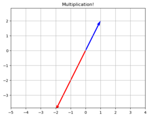
## add
z = v+w

print("The sum of v and w is ",z)

##Graphically:

## Tells Python to dray a blue arrow from (0,0) to (1,2)
plt.quiver(0, 0, v[0], v[1], color='b', units='xy', scale=1)
## and the red line is w
plt.quiver(v[0], v[1], w[0], w[1], color='b', units='xy', scale=1)
## and the sum
plt.quiver(0, 0, z[0], z[1], color='r', units='xy', scale=1)


plt.axis('equal')
plt.title('Adding makes sense geometrically!')

plt.xticks(range(-1,5))
plt.yticks(range(-1,5))


# Show plot with grid
plt.grid()
plt.show()
The sum of v and w is [4 3]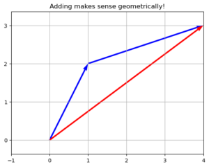
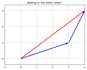
## order doesn't matter - that's important:


## add
z = w+v

print("Whe I flip the order, the sum is still ",z)

##Graphically:

## Tells Python to dray a blue arrow from (0,0) to (1,2)
plt.quiver(0, 0, w[0], w[1], color='b', units='xy', scale=1)
## and the red line is w
plt.quiver(w[0], w[1], v[0], v[1], color='b', units='xy', scale=1)
## and the sum
plt.quiver(0, 0, z[0], z[1], color='r', units='xy', scale=1)


plt.axis('equal')
plt.title('Adding in the other order!')

plt.xticks(range(-1,5))
plt.yticks(range(-1,5))


# Show plot with grid
plt.grid()
plt.show()
Whe I flip the order, the sum is still [4 3]
Getting super fancy:
I can combine these:
$$5 \binom{1}{2} - 3\binom{3}{1} =\binom{5-9}{10 - 3} = \binom{-4}{7}$$
## It's pretty easy to do this in Python.

5*v-3*w
array([-4, 7])Coordinate Representations
Remember [latex]\vec(v) = \binom{1}{2}[/latex] And how I said it was a set of directions? One step to the right, 2 steps up. We can write this using special vectors called Basis Vectors.
\[\binom{1}{2} = 1 \binom{1}{0}+ 2\binom{0}{1}\]
[latex]\binom{1}{0}[/latex] and $[latex]\binom{0}{1}[/latex] are basis vectors, which means that every 2-dimensional vector is a linear combination of there two.
But, there’s nothing actually that special about them. What do I mean? I can actually make any set of 2 vectors into a basis, as long as one isn’t a scaler multiple of the other. This is a trick that will come in handy later on.
Magnitude
We said that vectors have magnitude (length) and direction. We say that the length of the vector is the length of the line segment, and we can use Pythagorus. We use 2 lines (or one line) around a vector to show that we’re looking for it’s length.
\[ \left| \binom{a}{b}\right| =\sqrt{a^2+b^2}\]
Or:
\[\left|\binom{3}{4}\right| =\sqrt{3^2+4^2}=\sqrt{25}=5\]
This also works in other dimensions:
$$\left|\begin{pmatrix}1\\2\\
3\end{pmatrix}\right|=\sqrt{1^2+2^2+3^2} = \sqrt{14}\approx
3.7417$$
In linear algebra, we call this a Norm, and in
Machine Learning, it’s called the L2 Norm.
## This is much easier to do in python than to typeset the math!

## let's get some linear algebra things:

from numpy.linalg import *

a = np.array([3,4])
norm_a=norm(a)

print("The magnitude of vector ", a, "is ", norm_a)

b = np.array([1,2,3])
norm_b=norm(b)

print("The magnitude of vector ", b, "is ", norm_b)
The magnitude of vector [3 4] is 5.0
The magnitude of vector [1 2 3] is 3.7416573867739413The Dot Product
We’ve seen that we can add the vectors. and multiply a vector by a scaler. This leads to the question: Is there some form of multiplication between vectors? The answer is…. kind of.
In fact, there are two different kinds of multiplication-type operations: the dot product: (⃗v) ⋅ (⃗w) and The cross product: (⃗v) × (⃗w).
Definition:
The dot product is:
$$\begin{pmatrix}a\\b\end{pmatrix}\cdot
\begin{pmatrix}c\\d\end{pmatrix} = ac+ bd$$
This function takes in two vectors, and outputs a scaler (constant
number), for example:
$$\begin{pmatrix}1\\2\end{pmatrix}\cdot
\begin{pmatrix}3\\1\end{pmatrix} = (1)(3)+ (2)(1) =5$$
## this is again, easy in Python!

np.dot(v,w)

## And also for bigger arrays!

v1 = np.array([1,2,3,4])
v2 = np.array([4,-2,3,0])

v3= np.dot(v1, v2)

print(v1, " dot ", v2, " equals ", v3)
[1 2 3 4] dot [ 4 -2 3 0] equals 9Mathematically, the dot product is (kind of sort of) looking at the angle between the two vectors:
(⃗v) ⋅ (⃗w) = |(⃗v)||(⃗w)|cos θ
Where θ is the angle between the two vectors. What we really get out of this is:
If (⃗v) ⋅ (⃗w) = 0, than the two lines are perpendicular. That’s useful!
The Cross Product for completeness
The dot product is an operation which takes two vectors and returns a scalar. The Cross product is an operation which takes two vectors and
return another vector. It is defined specifically for 3-dimensional
vectors
The Cross Product:
$$\begin{pmatrix}a\\b\\c\end{pmatrix}\times
\begin{pmatrix}d\\e\\f\end{pmatrix} =
\begin{pmatrix}bf-ec\\cd-af\\ae-bd\end{pmatrix}$$
Hopefully, you look at that and think “Gee, I hope Python has a Cross Product function, because I don’t want to do that.” You would be correct.
In three dimensions, a⃗ × b⃗ is
orthogonal ( perpendicular) to both a⃗ and b⃗.
## It's just np.cross

v1 = np.array([1,2,3])
v2 = np.array([4,-2,3])

v3 = np.cross(v1,v2)

print(v1, " cross ", v2," equals ", v3)
[1 2 3] cross [ 4 -2 3] equals [ 12 9 -10]norm(v1-v2,1)7.0?norm