1 An Introduction
What is Economics?
You've heard of Principles of Microeconomics before. There is a lot of mathematics, the subject is abstract, but if you are like most students who sign up for Economics, you have no idea what Economics is. In this chapter we will attempt to answer the simple question of what Economics is. This chapter then introduces concepts that help understand what economists do (The Normative/Positive Dichotomy, Correlation, Causation, Experimental Design) and the definition of economics (Opportunity Cost and Opportunity Sets).
Example 1.1
Even though you still don't know the definition of Economics, let's start with a simple exercise. Can you guess which of the following questions falls under the purview of Economic research? Click on the question to find out the answer.
Most learners correctly claim that the first 3 issues fall under the umbrella of Economic research. However, they often mistakenly claim that one or more are not economic issues. All of these have been studied by economists: Gary Becker is the first economist to have published papers on the theory of marriage (Becker, 1973 & Becker, 1974), for example. Similarly, academics have studied climate change and we will use urban planning as an example in this chapter (See Example 1.10).
The Definition of Economics
“Economics is the science that studies how societies/individuals use limited resources to satisfy unlimited wants.”
Two important part of this definition are limited resources and unlimited wants. Limited resources imply that societies and individuals have a limited amount of resources available: from the moment we are born we are confronted with a limited resource, the time we have left to live. The idea that our wants are unlimited is more controversial. It implies that we have wants (material, emotional, physical, psychological etc.) and that these wants can never be completely satisfied. Some may claim that their wants are not unlimited. However, you must remember that wants are not only material, they include all wants. As such, while you may think that you have all the material goods that you need, wouldn’t you want more people to like you? Wouldn’t you want a more pristine and pollution free environment? Wouldn’t you want less inequalities, poverty or better healthcare? Hopefully, this gives you a better grasp of Economics and what it is. Introduction level textbooks in Economics usually focus on material wants. The focus on material wants makes the exposition easier and simpler. The rest of this textbook will thus ignore, in most cases, other types of wants.
Finally, Economics is a science. Before going further in our study of Economics it is useful to think about what that means. The next sections will thus explore what this means in more details.
The Normative/Positive Dichotomy
Statements about the world can be divided in two broad categories: Normative and Positive statements. Normative statements are statements concerning values. Normative statements are non-verifiable, we are unable to appeal to data to establish their accuracy. These statements will often, but not always, be phrased with should, ought to etc. On the other hand, Positive statements are statements of facts. Positive statements are verifiable, we can appeal to data to verify their truthfulness.
There are 2 common pitfalls that students should avoid when trying to identify the nature of a statement. First, positive statements are often mistaken to mean true. However, the requirement that a statement be verifiable does not imply that it has to be true. Secondly, we can easily craft verifiable assertions about normative statements. For example: “most economists believe X ought to be” is verifiable. We could survey economists and see if it is true that most economists agree. As such, it is positive.
Economists are scientists, they try to focus their attention on positive statements. Their goal is to identify the Economic laws that govern our world, what is and what isn’t. The purpose of Economics is not to make moral, or value, judgement about the world:
“Morality, it could be argued, represents the way that people would like the world to work – whereas economics represents how it actually does work.”
Levitt and Dubner, 2005
Science is science and ethics is ethics; it takes both to make a whole man; but only confusion, misunderstanding and discord can come from not keeping them separate and distinct.”
Friedman 1955
Economists can have personal values, ethical codes etc. However, these should be set aside when we analyze how the world is. The public often sees economists disagree in public, on TV or during public policy debates. Often, these disagreements arise because they do not share a common set of normative values. Despite these apparent disagreements, economists actually tend to agree on many topics. The topics on which economists have a broad agreement are usually topics for which economists would agree that the issue has largely been “resolved”. For example, on the benefit of trade or on the difference between cap-and-trade programs versus pollution (or Pigouvian) taxes (Both subjects you will learn about in this textbook).
Examples 1.3
The Chicago Booth School of Business has been asking questions to a panel of top ranked economic experts, the IGM Forum, for many years now. Broad agreement amongst economists can be found in answers to many of these questions:
1. The impact of the Trump administration’s steel and aluminum tariffs on Americans’ welfare.
2. All voting systems are flawed
3. Rising inequalities leads to less healthy democracies.
4. Investors are better off by investing in low cost index tracking ETFs than trying to beat the market.
5. Voters overestimate the impact of government policies on economic performance.
Obviously, not all of the questions on the IGM Forum see the panelists agreeing. In fact, the panelists do not seem to agree on most subjects.
Correlation and Causation
Now that we know that Economists tend to focus on positive statements, we need to pay attention to the distinction between causation and correlation:
- Causation: There is a causation between two variables when changes in one variable causes a change in another variable. For example, when the atmospheric pressure decreases, the boiling point for water decreases (Causation).
- Correlation: There is a correlation between two variables when the two variables move together but we can't say that one variable caused the other variable to change. Correlation can be caused by chance or a confounding variable. For example, when altitude increases, the boiling point of water decreases. Generally, when altitude changes, the atmospheric pressure decreases and that will cause the boiling point of water to change. Nevertheless, we can't say that altitude causes the boiling point of water to change. Suppose you fly in a pressurized airplane cabin at 35,000 foot. The atmospheric pressure in the cabin is equal to the atmospheric pressure at sea level. The boiling point at sea level and in the cabin would be the same: an increase in altitude does not cause the boiling point of water to increase.
Economics is often used to enlighten public policy design (how to make effective public policies). As such, causations are much more important to economists than correlations. If, for example, we want to design policies that increase income for the poorest households, we need to identify variables that causes earnings to increase (Education, for example). We can then design public policies that will affect the variables that will cause earnings to increase and attain our public policy goals. If however, we only know that 2 variables are correlated (let's say a specific employability social program and earnings), it is possible that implementing public policies based on this correlation will not attain the desired social outcomes.
There are different types of correlation and causation:
- Reverse Causation: Reverse causation arise when we believe that variable x causes variable y to change but variable y actually causes variable x to change. The causal link is the reverse of what we believed.
- Positive Correlation: An increase in variable x is accompanied by an increase in variable y.
- Negative Correlation: An increase in variable x is accompanied by a decrease in variable y.
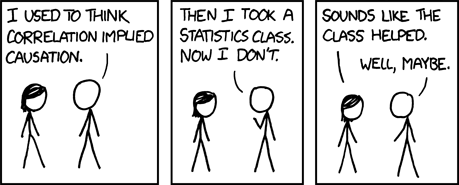
Finally, two variable that have a causal relationship will be correlated, but two variables that are correlated don't necessarily have a causal relationship. This leads to the famous statement: "Correlation doesn't imply causation."
Example 1.4
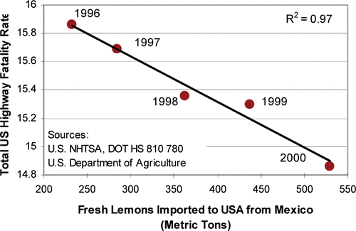
There is a link between the yearly US imports of lemon from Mexico and the number of fatalities as you can see in this Graph:
Is there a causation or correlation between these 2 variables?
The 2 variables seem to be correlated. When the imports of lemons increases, the number of road fatalities decreases. However, it is unlikely that there is any actual causal links between these variable. The link might just arise because of random chance. To be completely sure, we would need to investigate further. The next section will look at how economists can identify the causal relationship between variables.
Example 1.5
Consider the following graph that shows the relationship between the sales of ice cream (in Green) and the variation of weight compared to the average weight during the year (in Blue, +5 means the person weight 5 more pounds in that month compared to their yearly average weight):
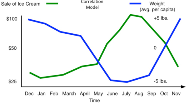
Your friend after seeing this graph concludes that if he wants to lose weight, he should buy more ice cream. The graph clearly shows that when sales of ice cream are higher, the weight is lower than the yearly average. Is the conclusion correct? What may be going on here?
The conclusion is incorrect. Remember, correlation does not imply causation! This is probably a problem of confounding variables, the weather/temperature affects both the level of activity that people do (and thus their weight) and the sales of ice cream. In June, July, August and September the weather is most likely nice, people do more physical activity and eat more ice cream. During months with bad weather, people stay inside, the sales of ice cream are lower and people's weight is higher.
Exercises
Experimental Design
Correlation is easy to find, but proving that we identified a causal effect is much harder. We want to identify the treatment effect: the effect of a treatment on those treated by it. In a perfect world, we would be able to observe the treated in 2 different universes. Both universes would be exactly the same, except that in one universe the treatment is applied and in the other universe the treatment is not applied. Obviously, we are unable to observe specific individuals in multiple universes. Instead. we measure the average treatment effect on the treated. Since we are unable to observe individuals in multiple different universes, we instead take 2 groups of individuals: the treatment and the control group. We apply the treatment to the treatment group and we use the control group as a way to measure what would happen to the treated if they had not been treated. This allows us to measure the average impact of the treatment on the treated. The most common way that scientists conduct such research is by using randomized controlled trials.
In order to measure the causal impact of the treatment properly, we need to make sure that our control group and experimental group are roughly the same. If the 2 groups are completely different, then the control group cannot serve as a valid proxy for what would happen to the experimental group if they didn't receive the treatment. Usually, we can get relatively similar control and experimental group by randomizing the members of each group.
Example 1.6
For example, if we give an experimental drugs (the treatment) to 1,000 mice (the experimental group), we may notice that 1 week later 10 mice passed away. We could conclude that the experimental treatment caused the 10 mice to die. However, death is a natural occurrence and mice will naturally die over time. To find out if the treatment actually caused the death, our only solution is to compare the treatment group with a control group. Suppose that we had another group of 1,000 mice. This other group was treated exactly the same as the experimental group but they didn't receive the experimental drug (they were given a placebo instead). If we notice that our control group also had 10 death, then maybe the experimental drug treatment was not responsible for the death in our experimental group.
To reinforce the importance of having comparable experimental and control groups: Suppose that the researchers only put healthy young mice in the experimental group and unhealthy old mice in the control group, would you still trust that the experimental drug is safe? Probably not, we would usually expect that healthy young mice die at a much slower rate then old unhealthy mice. To be able to trust the result of our experiment, we must make sure that both the experimental and control group are roughly the same.
What kind of experiments can we run in order to identify the causal link between 2 variables? Economists tend to use the following 3 types of experiments:
- Laboratory experiments: These experiments are similar to experiments in physics or health science. They are run in a laboratory with willing human participants (usually students). These are the easiest experiments to design. However, they suffer in their applicability to the real world: is an experiment run in a laboratory over a couple of hours really transferable to the real world? In health sciences or physics, probably. Maybe it's a bit harder to believe in the case of economic studies where we measure the response of the experimental group to different incentives.
- Field experiments: Are experiments that are designed by scientists, but instead of being run in a laboratory setting, the experiments are run in the real world. We might decide to offer different incentives for people to get their kids vaccinated in different villages in a developing country. We can then measure the impact of the incentives on the vaccination rate in the different villages. There is little doubt that the results from these experiments are applicable to the real world. They are, however, much more costly than laboratory experiments to run.
- Natural experiments: Different levels of governments consistently change public policies. These policy changes can be thought as experiments that the government is running all the time. Obviously, the elected government doesn't see these policy changes as an experiment but simply the correct policy to implement. However, economists can use these small policy changes as experiments to identify the causal impact of the policies by using clever experimental design. In Canada, Quebec is a gold mine for economists trying to identify the causal impact of policies. Quebec usually implements social policies at a different time than other jurisdictions. As such, it can often be used as a source of natural experiments (For example, Quebec started it's subsidized day care program in 1997, while most other Canadian jurisdictions didn't even contemplate such a program. We can use Canada as our control group and Quebec as our experimental group.).
Unfortunately, Economists are not always able to run controlled random trials (experiments) as easily as scientists in other hard sciences. There is a plethora of issues that plagues the design of controlled random trials in economics. We present 2 here: self-selection bias and moral issues:
- Self-selection bias: In many experiments that naturally arise in economics, the participants are able to self-selected into the treatment group or the control group. Suppose that you want to identify the impact of a training program on the probability of unemployed workers to find a new job. It is possible that only motivated unemployed workers apply to your program and that unmotivated workers do not apply to the program. When we measure the impact of the program on participants, we won't really know if any significant increases in the probability of finding a job was due to the program or the unobserved variables like motivation.
- Moral issues: Moral issues can often prevent economists from running experiments. We would like to know the impact of poverty on various outcomes, for example. It is immoral to force people to live in poverty just to measure such impacts though. This often limits the scope of the type of research that economists can run in the laboratory or in the field.
Empirical economics (running well designed experiments to evaluate the causal impact of a policy) takes a central role in modern economic research. Historically, economists themselves didn't believe that the experimental method could be applied in economics. However, things have changed a lot since:
In this course we will focus mostly on theoretical problems. The reason is twofold:
- In order to understand the empirical research that is conducted in economics a strong foundation in both statistics and economic theory is required.
- Theoretical models can give us useful intuitions that can be useful in multiple fields (business, finance etc.)
Choices and Costs
We have limited resources and unlimited wants; we have to choose how to use our limited resources! In fact, an alternative definition of economics could be: “The science that studies how individuals/societies make choices.” Fundamental to the economic thought process is the idea that every time you make a choice, you give up something. There is a cost to every single one of your decisions. For example, you are currently reading this textbook, you gave something up in order to read it. Perhaps you could be playing your favorite computer game, or having a beer with friends at the local pub. The cost of your decisions is the opportunity cost of your decision:
“The opportunity cost is the best forgone alternative.”
This definition implies that the opportunity cost is not an amount of money. The opportunity cost is what you gave up in order to get something. This cost will vary for each reader. If you did not buy (or do) something, what would you do instead?
Example 1.7
What is the opportunity cost of attending college? Presumably, if you are reading this textbook you are attending college or university. Identify the opportunity cost of your decision. Remember, the opportunity cost is not an amount of money, but for the purpose of this example, we will attempt to translate it into a monetary amount. Try to write down this opportunity cost now.
Answer:The opportunity cost of your college degree includes the money you spend on books and tuition. Normally, we would need to figure out what you would have done with that money but for the sake of simplicity we will just say that it cost you $8,000 a year for tuition and books. However, this is far from your only opportunity cost for attending college. While you are attending college, you have to spend a lot of time on school benches, or completing homework. What would you do with your time if you weren’t in college? Let’s assume that you would be working full time if you didn’t attend college and that you would earn roughly $35,000 a year. Are there any other opportunity costs to attending college? What about grocery or rent? These should not be included in your opportunity cost of attending college. You have to rent an apartment and buy grocery regardless of your decision to attend college.
When all is calculated the opportunity cost of your college degree is what you would do with the roughly $43,000 you are losing each year. You must value my time, lectures and textbook a lot to spend roughly $172,000 (about $43,000 a year times 4 years for a normal degree) for the privilege to learn what I have to teach. I am flattered!
Example 1.8
Imagine that Marcel spends all of his money on one of 2 different goods: French baguettes and bottles of wine. A bottle of wine cost $15 and a French baguette cost $3. What is the opportunity cost of a bottle of wine? What is the opportunity cost of a French baguette?
Answer:
To answer the first question, we have to find out what Marcel would do if he didn’t buy a bottle of wine. Since Marcel is assumed to spend all of his money on either wine or baguettes, we know that he would buy baguettes if he didn’t buy a bottle of wine. If he did not buy a bottle of wine, he would have $15 dollars available (The price of a bottle of wine), with that money he would be able to buy 5 baguettes ([latex]\frac{$15}{$3}[/latex] per baguettes). The opportunity cost of a bottle of wine is thus 5 baguettes.
To answer the second question, reverse the process. If he didn’t buy a baguette, he would have $3 (The price of a baguette), with that money he would be able to purchase 0.2 bottles of wine ([latex]\frac{$3}{$15}[/latex] per bottle of wine). The opportunity cost of a baguette is thus 0.2 bottles of wine for Marcel.
The astute reader might have noticed that the opportunity cost of a baguette is the inverse (1 divided by) of the opportunity cost of a bottle of wine ([latex]\frac{1}{5}=0.2[/latex]). This observation is always true. If the opportunity cost of a slice of pizza is 0.5 beer, the opportunity cost of a beer will be 2 slices of pizza (or [latex]\frac{1}{0.5}=2[/latex]).
The opportunity set is a graphical representation of 3 concepts that have been introduced thus far: Choice, Limited Resources and Opportunity Cost. To make this graphical representation, we simply graph the bundles that are attainable by a consumer/firm. Everything that is achievable is in the opportunity set and everything that is unachievable is outside of the opportunity set. Let’s demonstrate this concept with two examples.
Example 1.9
Marcel still only consumes one of 2 products: Wine or French baguettes. The price of a French baguette is $3 and the price of a bottle of wine is $15. Marcel has $30 available to spend on these 2 products. The opportunity set is a graph that represents all the possible bundles of French baguettes and wine he could purchase. The number of baguettes purchased by Marcel will be drawn on the X axis while the number of bottles of wine purchased by Marcel will be drawn on the Y axis. To complete the opportunity set ask yourself what different combinations of bottles of wine and baguettes Marcel could purchase:
| # of baguettes bought | Cost for baguettes | # of bottles of wine bought | Cost for wine | Total expense |
|---|---|---|---|---|
| 0 | $0 | 2 | $30 | $30 |
| 5 | $15 | 1 | $15 | $30 |
| 10 | $30 | 0 | $0 | $30 |
The previous table shows 3 possible bundles that Marcel could purchase with his $30. We can also graphically represent these bundles in a graph, this is the opportunity set:
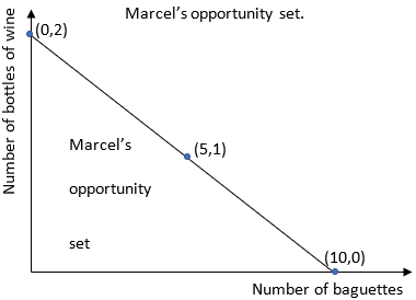
Example 1.10
The city of Victoria is currently reviewing the land use within the city. Land can be classified as “pristine untouched land” or as “land in use”. The first category comprises all the parks in the city and areas where nothing has been built yet. The second category comprises all the areas that are to be developed or have already been developed into residential, commercial or industrial zones. Assume that Victoria’s total land area is . We can represent this with the following opportunity set.
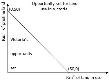
The frontier between the opportunity set and the points outside of it is important. Its name will vary depending on the application. If the opportunity set refers to a budget, as in the first example above, the frontier of the opportunity set is referred to as the budget constraint. When the opportunity set refers to the potential output of a firm or society, it is referred to as the production possibility frontier (or boundary).
All of the points that are in the opportunity set are said to be attainable. All of the points outside of the opportunity set are said to be unattainable. Points that are exactly on the frontier of the opportunity set, points that separate the attainable and unattainable points, are said to be efficient. These points are efficient because we are using all of the available resources. Points that are below the frontier between the opportunity set and the unattainable points are said to be inefficient.
Example 1.11
Taking Example 1.7:
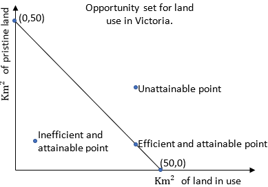
First, notice that the city of Victoria can choose to use all 50 of land as “pristine untouched land”. It could choose to use all 50 of land for commercial, residential or industrial use. Both choices are efficient, all our land is used.
The city could also decide to destroy all of the land in the municipality by pouring toxic waste all over it. It would use 0 square km as “pristine untouched land” and 0 square km for commercial, residential or industrial land. This would be an obvious waste of resources; it would be inefficient. Finally, some points are unattainable. The city cannot choose to have 30 square kms as pristine untouched natural land and 30 square kms as land in use. It only has 50 square kms available in total!
The opportunity set is a graphical representation of the limited resources of society because some points are unattainable. It is the graphical representation of choices because individuals or societies can only choose 1 point out of all the points in the opportunity set. Finally, it is the representation of the opportunity cost because the absolute value of the slope of the opportunity set is the opportunity cost of the good on the horizontal axis. This implies that the steeper the slope of the frontier of the opportunity set, the higher the opportunity cost of the good on the X axis is (Inversely, it implies a lower opportunity cost for the good on the Y axis).
Example 1.12
Let’s continue with the example in which Marcel had $30 and wanted to spend it all on wine and baguettes. A bottle of wine was priced at $15 and baguettes at $3. From example 1.5 we already know that the opportunity cost of a bottle of wine is 5 baguettes and the opportunity cost of a baguette is 0.2 bottles of wine. If we graph the opportunity set as in example 1.6, we get:
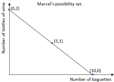
We can calculate the slope of the opportunity set by calculating: [latex]slope=\frac{rise}{run}[/latex]. The rise is the vertical distance between 2 points and the run is the horizontal distance. If we pick the points (0,2) and the point (10,0), we get [latex]\frac{(0-2)}{(10-0)}=\frac{-1}{5}[/latex]. In absolute value, this is exactly the opportunity cost of a baguette, the good on the horizontal axis.
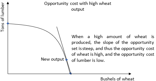
Production Possibility Frontiers are usually represented with a concave function. As more of a product is produced, the opportunity cost of that product increases: When a society is producing 0 units of wheat, the cost of producing wheat is relatively low. Workers with the best skills to produce wheat and the most favorable land to produce wheat can be shifted to wheat production. As more arable land and skilled workers are used to produce wheat, the country eventually runs out of workers with the relevant skills and/or arable land. The country may be able to produce more wheat, but the opportunity cost rises.
Example 1.13
Consider a country that only produces 2 goods: wheat and lumber. When the country produces a low amount of wheat, the slope is flat and opportunity cost for wheat is low.
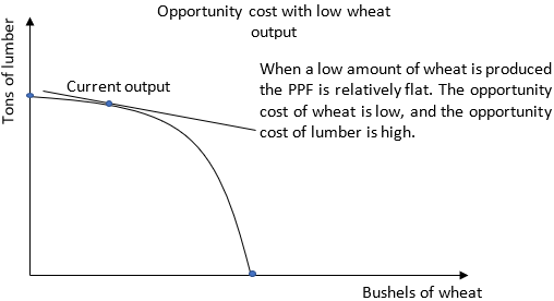
On the other hand, when the amount of wheat produced is high, the slope is steep and the opportunity cost for wheat is high.
