3 Demand, Supply and Markets
Introduction
Three concepts are introduced in this chapter. First, we introduce the supply curve, which is derived from the WTA. We then use the concept of WTP to define the demand curve. Finally, we combine the demand and supply curves together to form a market. Our purpose is to understand markets to do comparative static (analyze the impact of exogenous shocks on the price and quantity traded of goods) and the impact of government interventions.
The Supply curve
The supply curve is a relationship between the price of a good and the quantity that economic agents want to sell of that good. Usually the supply curve is represented in graphical form, but it can also be represented in algebraic form or in the form of a supply schedule.
There are two ways to think about the supply curve. One can think of the supply curve as how much money producers are willing to accept in order to produce and sell an extra good: it is the cost of producing another good. From the previous chapters, we know that the cost increases the more of a product a country, individual or firm produces (see the closing notes after example 2.5), this implies that the supply curve is upward sloping. The supply curve could also be interpreted this way: how many units would economic agents want to produce and sell at all possible prices.
Example 3.1
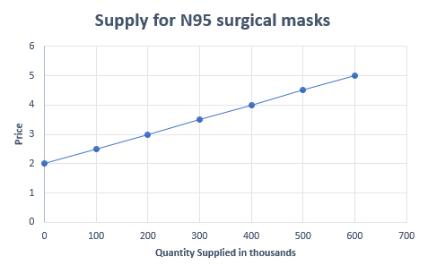
Let’s think about the supply of N95 surgical mask. The supply of N95 surgical masks is the quantity of mask that producers want to produce at every possible price for a given period, let’s say 1 year. Alternatively, we can think of the supply of N95 surgical mask as the price producers are willing to accept to produce an additional N95 surgical masks during a period of 1 year. We can represent the supply of N95 surgical masks in one of three different ways. First, as a graphical representation:
Second, as an algebraic formula:
[latex]P=2+0.005Q_s[/latex]; where [latex]P[/latex] is the price and [latex]Q_s[/latex] is the quantity supplied in thousands.
Third, as a schedule:
| Quantity supplied, yearly, of N95 masks | Price of Masks |
|---|---|
| 100 | 2.5 |
| 200 | 3 |
| 300 | 3.5 |
We won’t often use supply schedules, preferring the graphical or algebraic formula representation. However, it allows us to see clearly what the supply curve represents. When the price per mask is $2.5, firms would want to sell 100 thousand N95 masks per year. If the price per mask rises to $3, firms would want to sell 200 thousand N95 masks.
Example 3.2
This example demonstrate how to calculate the quantity supplied given a price. Suppose that the quantity supplied of gasoline is given by the following equation:
[latex]P=0.5+0.001Q_S[/latex]
P is the price per liter and the quantity is in thousands of liter per week.
Calculate the quantity of liters that would be supplied on this market if the price of a liter of gasoline is $1.5.
Answer:
To find the answer, we put the price of $1.5 in the supply curve:
[latex]1.5=0.5+0.001Q_S[/latex]
We then solve for the quantity demanded ([latex]Q_S[\latex]) in the previous equation.
[latex]1.5=0.5+0.001Q_S[/latex]; Minus 0.5 on both sides.
[latex]1=0.001Q_S[/latex]; divide both sides by 0.001
[latex]Q_S=\frac{1}{0.001}[/latex]
[latex]Q_S=1,000[/latex]
When the price is $1.5 per liter, [latex]Q_S[\latex] is 1,000. Since [latex]Q_S[\latex] is in thousands of liters, the quantity supplied is 1,000,000.
Shifts in the supply curve
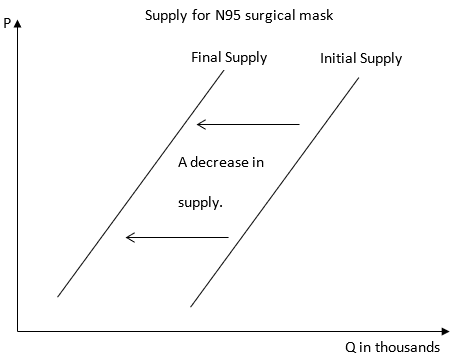
The supply curve shows the endogenous response of the quantity sold by producers to changes in the price (Or vice versa). An important question that arises is: “can other, exogenous, variables affect the supply of a good”. Since the supply curve is derived from the opportunity cost of producers, anything that can change the cost of production will affect the supply curve. Anything that reduces the cost of production will shift the supply curve to the right: as the cost of production decreases, producers are willing to produce more goods for a given price. This is called an increase in supply. When new producers join a market, the total supply of a good at any given price will increase. There are generally 3 exogenous shocks that can shift the supply curve to the right (left):
- Decrease (Increase) in the cost of inputs
- Improvement (Decrease) in technology
- Entry (Exit) of new producers
Example 3.2
Assume that we are considering the supply of N95 surgical masks, a type of mask used during surgical procedures. If new producers enter the market for N95 masks, we should see the supply curve moves to the right. If one of the many inputs for N95 masks: labour, pulp, machinery etc. sees their price increase, the supply curve will shift to the left. If we discover a new, cheaper method to produce N95 masks, the supply for N95 masks would shift to the right. 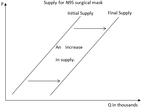
The Demand Curve
The demand curve is a relationship between the price of a good and the quantity that economic agents want to consume of that good. Just like the supply curve, the demand curve has 2 different interpretations. It can be interpreted as the quantity of goods that economic agents want to purchase for a given price in a given time period. It could also be described as the amount that economic agents are willing to pay in order to purchase an additional good. Ceteris paribus, the demand curve is downward slopping. The more units of a good consumed by economic agents, the lower their willingness to pay.
Example 3.3
The demand for N95 surgical masks is the quantity of masks that economic agents are willing to purchase in a given time period, say a year, at each given price. Alternatively, the demand for N95 surgical masks is the willingness to pay of economic agents to purchase one more surgical mask per year. The demand for N95 masks can be represented graphically: 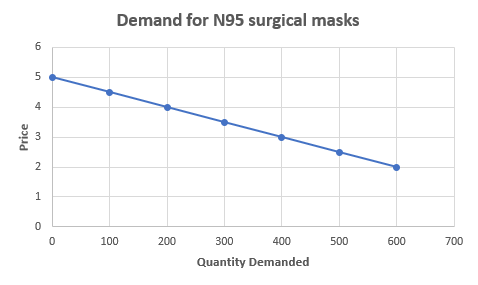 as an algebraic equation: [latex]P=5-0.005Q_D[/latex]; where [latex]P[/latex] is the price per box of 100 masks and [latex]Q_D[/latex] is the quantity of boxes demanded.
Finally, we can also represent the demand as a schedule:
| Quantity Demanded | Price |
|---|---|
| 0 | 5 |
| 100 | 4.5 |
| 200 | 4 |
Example 3.4
This example demonstrates how to calculate the quantity demanded given a demand curve and a price. Suppose that the quantity demanded of gasoline is given by the following equation:
[latex]P=5-0.001Q_D[/latex]
P is the price per liters and the quantity is in thousands of liters.
Calculate the quantity of gasoline that would be bought on this market if the price of a liter is $1.5.
Answer:
To find the answer, we put the price of $1.5 in the demand curve:
[latex]1.5=5-0.001Q_D[/latex]
We then solve for the quantity demanded ([latex]Q_D[/latex]) in the previous equation.
[latex]1.5=5-0.001Q_D[/latex]; Minus 1.5 on both sides and add [latex]0.001Q_D[/latex] on both sides
[latex]0.001Q_D=3.5[/latex]; divide both sides by 0.001
[latex]Q_D=\frac{3.5}{0.001}[/latex]
[latex]Q_D=3,500[/latex]
When the price is $1.5 per liter, the quantity demanded is 3,500 liters.
Utility and Marginal Utility
In order to understand why consumers’ willingness to pay decreases with the amount of good an economic agent consumes; it is useful to understand the concept of Utility and Marginal Utility. Economists assume that economic agents act as if they are trying to maximize a function: the Utility Function. You can think of it has a “welfare” or “happiness” function. The function takes as input everything in an economic agent’s life: the amount of milk he consumes per week, the quality of the water in his environment, their number of friends etc. The higher the value of this function, the happier or better off an economic agent is. Marginal utility is the increase in the utility of an economic agent when they consume one more unit of a given good. It is formally defined as the change in utility divided by the change in the quantity consumed of a good:
[latex]MU=\frac{\Delta TU}{\Delta Q_D}[/latex]; where [latex]\Delta TU[/latex] is the change in total utility and [latex]\Delta Q_D[/latex] is the change in quantity demanded.
Example 3.4
Consider Jie He, a student at Camosun College. She really likes steam buns and her utility, or welfare, depends on how many steam buns she eats during a week. The following table shows her utility and marginal utility when the quantity of steam buns consumed increases. On the right-hand side of the table is the marginal utility: by how much her utility increases every time she gets one more steam bun.
| # of steam buns | Utility | Increase in Utility (Marginal Utility) |
|---|---|---|
| 0 | 5326 | NA |
| 1 | 5335 | 9 |
| 2 | 5342 | 7 |
| 3 | 5345 | 3 |
The total utility and the quantity consumed are given. To calculate the marginal utility, we use the following equation: [latex]MU=\frac{\Delta TU}{\Delta Q_D}[/latex].
To find the marginal utility for the first steam bun consumed we calculate:
[latex]MU=\frac{5335-5326}{1-0}=9[/latex]
To find the marginal utility for the second steam bun consumed we calculate:
[latex]MU=\frac{5342-5335}{2-1}=7[/latex]
Economists make assumptions about the utility function:
- The Utility Function is monotonous. This means that the utility function is increasing in all of its arguments: if people get more of anything their utility increases.
- Decreasing Marginal Utility: the increase in utility provided by each new good consumed is smaller than the increase provided by the previous unit of the same good.
Sometimes students disagree with the first assumption. They’ll claim for example that water pollution causes negative impacts on individuals and that an increase in pollution shouldn’t increase “welfare” or utility. The answer to this objection is that we can redefine the inputs of the utility function so that an increase is considered beneficial. Instead of considering water pollution as an input to the utility function, we can consider water quality to be an input.
Why is marginal utility decreasing? When we purchase a good for a second, third time etc. the need that the good satisfies has already been satisfied to some extent. As such, each new unit of the good brings us less satisfaction then the previous unit consumed. Imagine something that you like, like puppies or cars. If you get a first puppy, the first puppy gives you a lot of happiness or utility. The second puppy will increase your happiness, but probably not by as much as the first puppy. You have to be aware, that we are considering comparable good. If your first car is an old used car, and you then purchase a luxury car, it is possible that the second car brings you as much, or more, happiness than the first car. However, in this case you are not consuming more of the same good, you are consuming a different good.
Example 3.5
Here is Jie's utility again:
| # of steam buns | Utility | Increase in Utility (Marginal Utility) |
|---|---|---|
| 0 | 5326 | NA |
| 1 | 5335 | 9 |
| 2 | 5342 | 7 |
| 3 | 5345 | 3 |
When Jie consumes 0 steam buns, her utility is positive. Presumably, because she consumes other goods. When she consumes more steam buns, her utility increases. This is the first assumption: utility is increasing. As you can see in the last column, the rate of increase in her utility is decreasing. The reason her marginal utility is decreasing is because of the diminishing marginal utility assumption.
Shifts in the Demand Curve
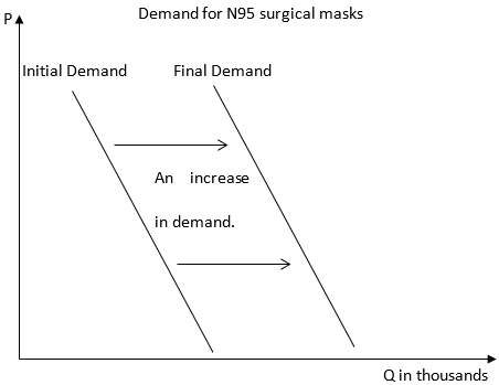
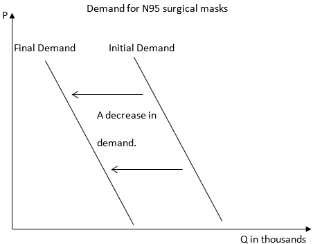
The Demand curve shows the endogenous response of the quantity demanded to changes in the price level (or vice versa). However, just like with the supply curve, exogenous variables can lead to shifts in the demand curve. Anything that would cause consumers to want to purchase more of the good, at any given price level, will cause the demand curve to shift right, called an increase in Demand. Shocks that would cause consumers to want to purchase less of the good, at any price level, will cause the Demand curve to shift left, a decrease in Demand.
Examples
Increase in Demand:
Decrease in Demand:
Here are the most common exogenous shocks that can shift the demand curve:
- Increase in income
- Changes in consumer preferences
- Changes in the price of other goods
- Expectations about the future
The impact of some of these changes can be ambiguous. The effect of an increase in income on the demand curve depends on the nature of the good that we are talking about. If the good is a normal good, an increase in income would lead to an increase (shift right) of the demand curve. However, if the good is an inferior good, an increase in income would lead to a decrease (shift left) of the demand curve. Inferior goods are goods that consumers usually consume because they are poor, as they get richer, they substitute away from these goods and consume other goods instead. Consider for example Kraft Diner, as the income of a consumer increases, they are less likely to consume Kraft Diner and more likely to increase consumption of other goods, like restaurant meals. When income increases, demand for Kraft Diner decreases. Normal goods, are the vast majority of goods. When income increases people want to increase consumption of normal goods. Restaurant meals, as discussed above, would be an example of a normal good.
Many things can change the preferences of consumers: successful marketing campaign, new research or knowledge etc. When consumers’ preference for a good increase, the demand curve shifts right. When consumers’ preference for a good decrease, the demand curve shifts left.
When the price of another good changes it can lead to a change in the demand for this good. The impact will depend on whether the other good is a substitute or a complement. Complements are goods that people tend to consume together: they complement each other. Substitutes, on the other hand, are two goods that satisfy the same desire or want. As such, consumers usually only consume one or the other, but not both at the same time. An increase in the price of a substitute would lead to an increase in the demand for the good we are looking at. Since it has become more expensive to satisfy our want with the substitute, economic agents will turn to the good we are analyzing instead. The demand will increase and the demand curve will shift right. In the case of a complement, the opposite effect would happen. If the price of a complement increases, people will be less likely to consume the good that we are analyzing, as it will now be more expensive to satisfy our want. The demand curve will shift left; the demand will decrease.
Finally, expectations about the future can also have an impact on the demand for a good. When people believe that the price of a good will increase in the future, they are more likely to want and purchase the product now. If people expect the demand to decrease in the future, the demand will decrease now.
In summary, here are all of the exogenous shocks that can lead to an increase (decrease) in the demand for a product (Good X):
- Change in income:
- An increase (decrease) in income for a normal good, will lead to an increase (decrease) in demand.
- A decrease (increase) in income for an inferior good, will lead to an increase (decrease) in demand.
- Change in preferences:
- An increase (decrease) in preference, will lead to an increase (decrease) in demand.
- Change in the price of another good (Good Y):
- If Good Y is a substitute, an increase (decrease) in the price of Good Y, will lead to an increase (decrease) in demand for Good X.
- If Good Y is a complement, a decrease (increase) in the price of Good Y, will lead to an increase (decrease) in demand for Good X.
- Expectations about the future:
- If consumers expect that the price of a product will increase (decrease) in the future, it will lead to an increase (decrease) in demand for Good X.
This list of exogenous shocks that can shift the demand curve is not exhaustive, but it covers the most frequent shocks that can affect the demand curve.
Example 3.7
Demand and Income:
Consider the demand for cars. Cars are a normal good. When the income of consumers increases, they will want to purchase more cars and the demand for cars will increase, or shift to the right.
Now, consider the demand for instant noodles. Instant noodles could be considered an inferior good. As people become richer, they are less likely to purchase instant noodles, substituting instant noodles for restaurant meals or other alternatives. As such, when the income of consumers increases, the demand for instant noodles will decrease, or shift left.
Demand and Preferences:
Consider the demand for orange juice. Suppose that new research shows, without any doubt, that daily consumption of orange juice reduces the risk of cancer and extend consumers’ lives. It is likely people will want to consume more orange juice, the demand for orange juice increases, or shift to the right.
Demand, substitutes and complements:
If we think about the demand for ketchup, which is a complement to fries, we should see that if the price of fries increases, the demand for ketchup should decrease. People like to eat fries and ketchup together but if fries are more expensive, they are less likely to buy fries and ketchup.
On the other hand, if the price of strawberries increases, we would expect that the demand for blueberries, a substitute to strawberries, increases. If people can’t satisfy their desire for small fruits by eating strawberries because they are more expensive, people are more likely to buy blueberries instead.
Expectations about the future and Demand:
Finally, consider the demand for houses. Suppose that people expect that the price of houses will increase in the future. If this is the case, they are more likely to purchase houses right now, to avoid paying a high price in the future. The demand for houses would go up immediately.
Market and Market Equilibrium
A market is not necessarily a physical place. A market is comprised of 3 important elements: buyers, sellers and a mean for them to connect. There are a lot of different types of markets. The different types of markets are usually divided by the market power that different agents have on the market or the number of buyers or sellers. Typically, the two are pretty similar. When there is a lower amount of sellers on a market, each seller has more power. When there is a higher amount of sellers on a market, each seller has more power. We usually divide the different types of market in the following catefories:
- Monopsony: One buyer and multiple sellers, the buyer has a lot of market power.
- Perfect Competition: A lot of buyers and a lot of sellers, neither buyers or sellers have any power.
- Monopolistic Competition: A lot of buyers and a lot of sellers, each sellers has some market power.
- Oligopoly: A lot of buyers and a small amount of sellers, each seller has significant market power.
- Monopoly: A lot of buyers and a single seller, the seller has a lot of market power.
For this section, we will assume that the markets are in perfect competition. This is the "base" case in Economics. This does not mean that this is the most common market structure.
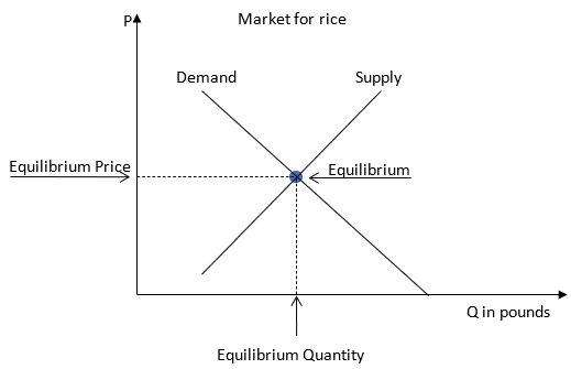
In a market in Perfect Competition, the buyers on the market are represented by the demand curve: the quantity that people want to buy at every possible price. The sellers on the market are represented by the supply curve: the quantity that people want to sell at every possible price. They can connect in many different ways: in a physical location, online etc. On each market, a market equilibrium will naturally arise. In the case of perfect competition, the market equilibrium is located at the intersection of the demand and supply curves. The equilibrium price and the equilibrium quantity are the price and quantity that should arise on this market. Here is a graphical representation:
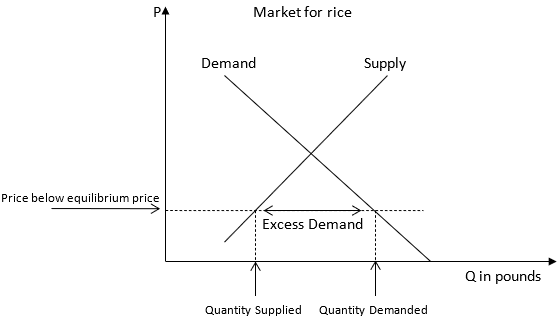
If the price was below the equilibrium price, consumers would want to purchase more goods than suppliers are willing to sell: There would be excess demand (Quantity demanded > Quantity supplied). Here is a graphical representation of a market in which there is excess demand:
If the price was above the equilibrium price, suppliers would want to sell more goods than consumers are willing to purchase: There would be excess supply.
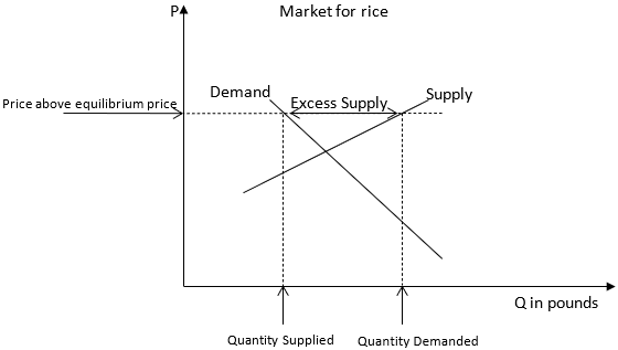
There are 2 types of equilibriums, stable and unstable equilibriums. The natural forces around a stable equilibrium push back towards the equilibrium. The easiest way to visualize this, is to think about a punching bag. If you hang one from the ceiling of your house, it will stay in one position and won’t move, this is the equilibrium. If you were to disturb it, by punching or kicking the bag, it would move. However, the natural forces around the equilibrium push back towards its initial position. As such, once you stop punching, the bag will go back to the initial position, a stable equilibrium. An interesting element of stable equilibriums is that they are much more likely to arise naturally. If you left for 2 months, you would naturally expect to find your punching bag in the same position you left it in. The natural forces around an unstable equilibrium push away from the equilibrium. You can visualize one of these equilibrium by thinking about a quarter that his holding on its side, it is neither on head nor tail. It is possible for a quarter to be placed, or even to randomly end, in this position but natural forces push away from it. If you were to disturb the equilibrium, the quarter would fall in a new equilibrium, either on head or tail. These equilibriums are mathematically interesting, but all equilibriums we will introduce in this book are stable, we expect these equilibriums to arise naturally much more frequently than unstable ones. Some equilibriums are a mix of stable and unstable equilibriums, but we won’t discuss these here.
The market equilibrium is a stable equilibrium. If the price level is above the equilibrium price, natural forces will push it back down. If it was below the equilibrium price, natural forces would push it back up. These pressure on the price level are the result of excess demand or excess supply. When there is excess demand, some consumers of the good are unable to purchase it. They go to many different stores; they look online and all firms are sold out. When they try to order the good from a local retailer, they learn that it will take months to receive the product because the list of people who already ordered the product is long. Some of the consumers that can’t find the product are willing to pay a higher price then the current one. These consumers will offer a higher price to the retailer in order to get to the top of the list and receive their product first: Excess demand leads to an increase in the price level.
Example 3.8
This example asks you to identify the natural forces that would push the price back to equilibrium if it was off equilibrium:
Example 3.9
Given an algebraic equation for the demand and supply of a product, you should be able to solve for the equilibrium quantity and price. Suppose that the demand curve is given by [latex]P=25-2Q_D[/latex] and the supply curve is given by [latex]P=5+3Q_S[/latex], where the quantities are in thousand of units per week.
Can we find the equilibrium price and quantity? Looking at the graph, we can see that the quantity demanded and the quantity supplied should be the same at the equilibrium and that the price on both the demand and supply curve should also be the same. This information tells us that:
- [latex]Q_S=Q_D=Q^E[/latex]; where [latex]Q^E[/latex] is the equilibrium quantity
- [latex]P^E[/latex] is such that [latex]25-2Q_D=5+3Q_S[/latex]; where [latex]P^E[/latex] is the equilibrium price
We can use this information to solve the system of equation. Using the fact that [latex]Q_S=Q_D=Q^E[/latex] we can replace [latex]Q_S[/latex] and [latex]Q_D[/latex] in the equation given in 2 and solve for [latex]Q_E[/latex]:
[latex]25-2Q^E=5+3Q^E[/latex]
[latex]20=5Q^E[/latex]; by adding 5 on both side and adding [latex]2Q^E[/latex] on both sides
[latex]\frac{5}{20}=Q^E[/latex]; by dividing both sides by 5
[latex]4=Q^E[/latex]
Once we know [latex]Q^E[latex], we can substitute it in either the demand curve or the supply curve:
In the supply curve: [latex]P=5+3Q_S=5+3\times4=17[/latex]
In the demand curve: [latex]P=25-2Q_D=25-2\times4=17[/latex]
Notice that it is irrelevant if we use the supply or the demand curve to find the equilibrium price. They both give the same result. However, it is a good habit to use both the supply and demand curve to find the equilibrium price. Simply put, it allows you to verify that your answer is the right one. If your answer using the supply and demand curve are different, you know that you made a mistake somewhere.
Comparative Static
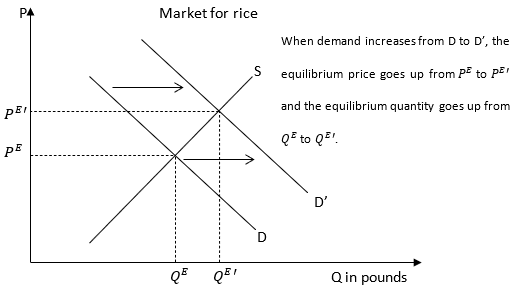
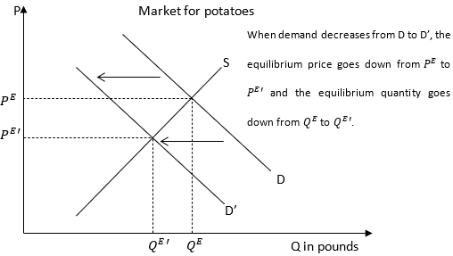
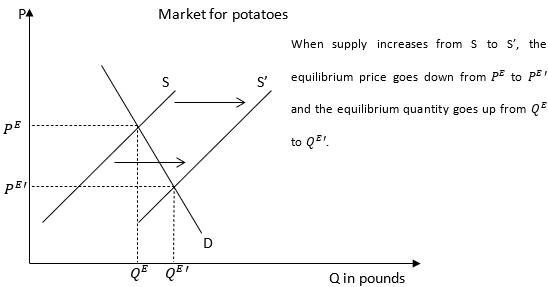
When a market is in equilibrium, exogenous shocks may arise and disturb the initial equilibrium. These shocks arise when exogenous variables shift the demand or supply curve. Analyzing the impact of these exogenous changes on the equilibrium price and quantity is called comparative statics. Economists use it to predict the impact of changes in exogenous variables on the equilibrium price and quantity. Simply draw the graph for the given market and look at what happens visually. I provide the 4 possible cases below:
An increase in demand will cause the equilibrium price and quantity to increase:
A decrease in demand will cause the equilibrium price and quantity to decrease:
An increase in supply will cause the equilibrium price to decrease an the equilibrium quantity to increase:
A decrease in supply will cause the equilibrium price to increase and the equilibrium quantity to decrease:
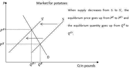
Examples
Question: What is the impact of a simultaneous increase in demand and supply on the equilibrium price and quantity?
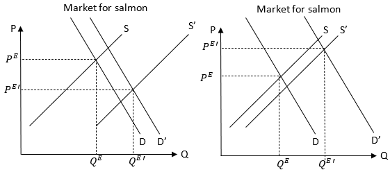
Answer: The quantity sold on this market will increase since both the demand and supply shift right. However, in this specific case it is uncertain what will happen to the price. The previous graphs shows that the price could go up or down (it could also stay unchanged) depending on how far the demand and supply move to the right. In the first graph, the price decreases. In the second graph, the price increases.
Conclusion
We now have the basics tools that allow us to understand what will happen following different exogeneous changes in income, quantity of suppliers etc. Armed with this knowledge, we are ready to analyze the impact of government policies: are they effective? The following 2 chapters will discuss government intervention thoroughly. As we move forward, remember that chapter 4 will make the right-wing argument against market intervention. While chapter 5 will make the left-wing argument for market intervention. The argument for free markets is not introduced first for ideological reasons. It is introduced first because of historically considerations and it is, admittedly, simpler than the argument for government intervention.
