Climatic & Ecological Modelling for Adaptive Forest Applications by Dr. Tongli Wang is licensed under a Creative Commons Attribution-NonCommercial-NoDerivatives 4.0 International License, except where otherwise noted.
“Climatic & Ecological Modelling for Adaptive Forest Applications” by Dr. Tongli Wang, University of British Columbia, Adaptation Learning Network is licensed under CC BY NC ND except where indicated. For external links to resources, review the rights and permission details.
1. Weather and climate
2. Extreme events
3. Climate change and climate variability
3.1. Climate change
3.2. Climate variability
3.3. EI Nino Southern Oscillation (ENSO)
3.4. Possible changes in mean and variance
4. Observed climate change
4.1. Observed changes in average temperature
4.2. Observed changes in mean and variance of temperature
4.3. Observed changes in ice caps in the arctic
4.4. Observed changes in sea level
5. Causes of climate change
5.1. Greenhouse gases
5.2. The role of human activity
5.3. Solar irradiance
6. Future projections of climate change
6.1. Projections of fossil fuel emission
6.2. Projections of global temperature
7. Mitigation and adaptation to climate change
7.1. Mitigation to climate change
7.2. Adaptation to climate change
Summary
Before we talk about climate change, we first need to be clear about the definition of climate and the difference between climate and weather.
Weather is the state of the atmosphere at a place and time as regards temperature, precipitation, humidity, cloud, wind, etc. Weather is different in different parts of regions (as illustrated in Figure 1) and the world and changes over minutes, hours, days, and weeks.
Climate, on the other hand, is about the statistics of weather over long periods of time including averages, extremes, timing, the spatial distribution of weather attributes as mentioned above. The period is typically 30 years – a normal period, as shown in Figure 2. We refer to these 30-year averages of weather observations as climate normals. The reference normal period is 1961-1990 defined by the World Meteorological Organization (WMO).
The difference between climate and weather is best summarized by the popular phrase: “the Climate is what you expect; the weather is what you get” – Mark Twain
Weather and climate extremes such as hurricanes, tornadoes, heavy downpours, heat waves, and droughts affect all sectors of the economy and the environment, impacting people where they live and work. Extreme events also include unexpected, unusual, unpredictable, severe or unseasonal weather, or weather events at the extremes of the historical distributions as illustrated in Figure 3. Extreme weather events are considered as climate components.
For a given location, we expect the weather to change a lot from day to day, month to month, and year to year (Figure 4, left). In contrast, we expect the climate to remain relatively constant. If the climate doesn’t remain constant, as shown in Figure 4 (right), we call it climate change. It is important to distinguish between short-term variability and long-term climate change.
Climate variability is defined as variations in the mean state and other statistics of the climate on all temporal and spatial scales, beyond individual weather events. The term “climate variability” is often used to denote deviations of climatic statistics over a given period of time (e.g. a month, season or year) when compared to long-term statistics for the same calendar period, as shown in Figure 5. Climate variability is measured by these deviations, which are usually termed anomalies.
Climate variability may be due to natural internal processes within the climate system (internal variability), or to variations in natural or anthropogenic external factors (external variability). Climate variability and climate change can occur independently, but they can also occur at the same time. The main driver of climate variability in Pacific region is EI Nino Southern Oscillation (ENSO).
ENSO is an irregularly periodic variation in winds and sea surface temperatures over the tropical eastern Pacific Ocean, as shown in Figure 6. It affects the climate of much of the tropics and subtropics. The warming phase of the sea temperature is known as El Niño and the cooling phase as La Niña.
The El Niño and La Niña phenomenons are well explained in these two short videos:
A Youtube video from usoceangov
A Youtube video from Met Office – Weather
For temperature, climate change may result in an increase in mean, variance, or both mean and variance as illustrated in Figure 7. If climate change results in an increase in mean temperature only, the distribution of the probability of occurrence of temperatures would shift to the right without changing the shape of the distribution (Figure 7a).
If climate change results in an increase in variation of the temperature only, the temperature distribution would not shift, but the shape of the distribution would become flatter and wider, resulting in greater probabilities of extreme events (Figure 7b).
If climate change results in an increase in both mean and variation of the temperature, the temperature distribution would shift right and the shape of the distribution would become flatter and wider, resulting in greater probabilities of extreme events in the hot end (Figure 7c).
For precipitation, the change may be more obvious for variance than for mean, resulting in less probability of occurrence in light precipitation and more in heavy precipitation (Figure 8).
Climate change has been observed over the last three decades. Due to annual fluctuation (Figure 9, upper), the trend of climate change is more obvious when organized in decadal averages (Figure 9, lower).
The change in temperature is even more evident in the current decade of 2011 – 2018 (Figure 1.1.10), which is not included in Figure 1.1.9.
Observations of the temperature of Northern and Southern Hemisphere land areas (James Hansen and Makiko Sato, 2016) show that distributions of temperature both shifted to the right (increased in mean) and flattened (increased in variance) over the last decades. The increases in variance in summer months are greater than in winter months. The increase in both mean and variance suggests an increase in the extremely hot temperatures.
The effects of climate change in the Arctic include rising air and water temperatures, loss of sea ice. Sea ice is currently in decline in area, extent, and volume. Sea ice area refers to the total area covered by ice, whereas sea ice extent is the area of ocean with at least 15% sea ice, while the volume is the total amount of ice in the Arctic.
In 1984 the sea ice extent (Figure 12, lower) was roughly the average of the minimum from 1979 to 2000, and so was a typical year. The minimum sea ice extent in 2012 was roughly half of that average (Figure 12, upper).
Climate change is causing a continuous increase in sea level. Sea level rise is caused primarily by two factors related to global warming: the added water from melting ice sheets and glaciers and the expansion of seawater as it warms. The graph in Figure 13 shows the change in sea level since 1993 as observed by satellites.
Certain gases in the atmosphere block heat from escaping, causing “greenhouse effect”, thus named as greenhouse gases. Long-lived gases that remain semi-permanently in the atmosphere and do not respond physically or chemically to changes in temperature are described as “forcing” of climate change (i.e., climate change forcing factors). Gases, such as water vapor, which respond physically or chemically to changes in temperature are seen as “feedbacks.”
Gases that contribute to the greenhouse effect include:
Water vapor. The most abundant greenhouse gas, but importantly, it acts as a feedback to the climate. Water vapor increases as the Earth’s atmosphere warms, but so does the possibility of clouds and precipitation, making these some of the most important feedback mechanisms to the greenhouse effect.
Carbon dioxide (CO2). A minor but very important component of the atmosphere, carbon dioxide is released through natural processes such as respiration and volcano eruptions and through human activities such as deforestation, land-use changes, and burning fossil fuels.
Methane. A hydrocarbon gas produced both through natural sources and human activities, including the decomposition of wastes in landfills, agriculture, and especially rice cultivation, as well as ruminant digestion and manure management associated with domestic livestock. Methane is a far more active greenhouse gas than carbon dioxide, but it is much less abundant in the atmosphere.
Nitrous oxide. A powerful greenhouse gas produced by soil cultivation practices, especially the use of commercial and organic fertilizers, fossil fuel combustion, nitric acid production, and biomass burning.
Humans have increased atmospheric CO2 concentration by more than a third since the Industrial Revolution began. This is the most important long-lived “forcing” of climate change. The carbon dioxide data, measured as the mole fraction in dry air, show a rapid rise since 1958 and hit the record high in 2019 (Figure 15).
Figure 15. Changes in CO2 level since 1958. Credit: Scripps Institution of Oceanography (in public domain). Source: https://scripps.ucsd.edu/programs/keelingcurve/co2-graphs/In its Fifth Assessment Report, the Intergovernmental Panel on Climate Change (IPCC), a group of 1,300 independent scientific experts from countries all over the world under the auspices of the United Nations, concluded there’s a more than 95 percent probability that human activities over the past 50 years have warmed our planet.
As shown in Figure 16, the amount of solar irradiance did not increase over the past half-century. Thus, it is extremely unlikely that the sun has caused the observed global temperature warming trend over this period.
These are four scenarios produced by the IPCC to span a range of emissions trajectories for this century (Figure 17). These scenarios are called Representative Concentration Pathways (RPCs). A Representative Concentration Pathway (RCP) is a greenhouse gas concentration (not emissions) trajectory adopted by the IPCC for its fifth Assessment Report (AR5) in 2014. Four pathways have been selected for climate modeling and research. They describe different climate futures, all of which are considered possible depending on the volume of greenhouse gases (GHG) emitted in the years to come. The four RCPs, namely RCP2.6, RCP4.5, RCP6, and RCP8.5, are labeled after a possible range of radiative forcing values (i.e., incoming energy – outgoing energy) in the year 2100 (2.6, 4.5, 6.0, and 8.5 W/m2, respectively). RCP8.5 is often referred to as a ‘business as usual’ pathway, while RCP2.6 requires immediate and drastic action to start reducing global CO2 emissions before 2020.
For the “business as usual” emission scenario RCP 8.5, the projected global temperature increases by 2100 will be about 6°C on average (Figure 18). Even with the aggressive mitigation scenario RCP2.6 requiring immediate and drastic action, the projected increase will be about 1.5°C by the end of the century, which is the target of the Paris Agreement.
The following maps in Figure 19 show the spatial pattern of the temperature increase and comparisons between the two scenarios RCP 2.6 and RCP 8.5.
Mitigation and adaptation are the two major approaches to fight against climate change. Mitigation measures are to reduce or prevent the emission of greenhouse gases into the atmosphere; while adaptation actions are to reduce the negative impact of climate change and to take the advantage of potential new opportunities.
Mitigation addresses the root causes while adaptation seeks to lower the risks due to climatic changes. Despite various mitigation measures, climate change is inevitable. Thus, actions for adaptation are required regardless of greenhouse-gas emission scenarios.
The following are possible measures for climate change mitigation:
The following are possible activities to adapt to climate change:
Weather changes a lot day by day, but we expect that climate remains constant for the same time of the year. Climate variability refers to short-term variation while climate change is a change in a long-term trend. Climate change has been observed with shifted mean increased probability of extremes. The main cause of climate change is anthropogenic emissions of greenhouse gases (GHGs). Projected future climates based on a range of GHGs emission scenarios are threatening. Climate change mitigation and adaptation are the two options to fight against climate change, and forest ecosystems play important roles in both.
1. Forest ecosystems
1.1. Definition of a forest ecosystem
1.2. Distribution of forest ecosystems
1.3. Biomes
1.4. Classification of forest ecosystem
1.5. Functions of forest ecosystems
2. Impacts of Climate Change on Forest growth and productivity
2.1. Positive impact on forest growth and productivity
2.2. Negative impact on forest growth and productivity
3. Impacts of Climate Change on the vulnerability of forest ecosystems to pests and diseases
3.1. Impacts on the vulnerability of forest ecosystems to pests
3.2. Impacts on the vulnerability of forest ecosystems to diseases
4. Impacts of Climate Change on forest fires
5. Impacts of Climate Change on biodiversity and sustainability of forest ecosystems
5.1. Impacts on biodiversity
5.2. Impacts on sustainability
6. Impacts of Climate Change on Forest Ecosystems’ services
6.1. Effects on water quantity and quality
6.2. Impact on recreation provided by forest ecosystems
7. Mitigation of climate change by forest ecosystems
7.1. Carbon sequestration
7.2. Renewable materials
Summary
A forest ecosystem is a terrestrial unit consisting of plants, animals and micro-organisms (biotic components), all interacting among themselves and with the environmental (abiotic) factors including soil, climate, water, and light. The organisms involved in a forest ecosystem are interdependent on one another for survival and can be broadly classified according to their ecological role as producers, consumers, and decomposers. Healthy forest ecosystems are usually self-sustaining. Larger ecosystems with wide diversity are much more stable and resilient to harmful changes.
The world’s total forest area in 2010 is estimated to be just over 4 billion hectares, occupying 31% of the world land areas, and corresponding to an average of 0.6 ha of forest per capita. The five most forest-rich countries (Russia, Brazil, Canada, the United States of America, and China) account for more than half of the total forest areas (53 percent). For detail, please read the FAO report at http://www.fao.org/3/i1757e/i1757e02.pdf.
A biome is a specific geographic area of the planet that can be classified according to the plants and animals that live in it. Temperature, soil, and the amount of light and water help determine what life exists in a biome.
Classification of biomes provides a basis for forest ecosystem classification. However, not all scientists classify biomes in the same way. Some scientists use broad classifications and count as few as six biomes. These are forest, grassland, freshwater, marine, desert, and tundra. Others use more precise classifications and list dozens of different biomes. For example, they consider different kinds of forests to be different biomes, as shown in Figure 3. Tropical rain forests that are warm and wet year-round are one biome. Temperate deciduous forests—those that have cold winters, warm summers, and are dominated by trees that lose their leaves—are a different biome. Taiga forests, which are in cold regions and are dominated by cone-bearing firs and spruces, are yet another biome.
Biomes move as the climate changes. Ten thousand years ago, parts of North Africa were lush landscapes cut by flowing rivers. Hippopotamuses, giraffes, and crocodiles lived amid abundant trees. Gradually, the climate dried out. Today, this region is part of the Sahara Desert, the world’s largest desert.
Forest ecosystem classification is often in a hierarchal system, from a landscape level at the top and to a site level at the bottom. Forest ecosystems can be classified according to the type of biome in which they exist, particularly for the classification at the landscape level.
At a landscape level, Forest ecosystem classification provides a framework for landscape analysis and planning. It is based on features such as climate, elevation, topography, bedrock formation, and vegetation. For example, the Biogeoclimatic Ecosystem Classification (BEC) divides British Columbia into 16 zones (Figure 4).
At a stand level, classifying forest ecosystems is based on vegetation, soil, and site attributes, which allows users to recognize similar ecosystem units on the ground and to develop a common strategy for forest resources management.
A forest ecosystem is often named by the primary tree species that form the canopy of the system. For example, the Coastal Douglas-fir forest ecosystem in North America (Figure 3), and Chinese pine forest ecosystem in China.
In the past, timber production was regarded as the dominant function of forests. In recent years, however, this perception has shifted to include other forest functions and services, such as:
These will be covered in more detail later in this topic.
In the short term, increased temperature and prolonged growth periods (Figure 6) may improve tree growth in cooler regions for some period, where temperature is a limiting factor for tree growth.
Elevated CO2 concentration may promote the photosynthesis rate. Such an effect may increase under warmer temperature as shown in the graph of Figure 7.
Figure 7. Photosynthetic response to CO2 concentration, shown at four temperatures, based on calculations for RuBP regeneration-limited photosynthesis. Image by Kirschbaum (2011). Open access source: http://www.plantphysiol.org/content/155/1/117Elevated CO2 concentration may also promote water use efficiency. Plants take in carbon dioxide and lose water vapor through stomata. Under elevated carbon dioxide levels, the stomata need to open smaller and the plant loses less water.
In the long term, climate change will cause a mismatch between the climate that a tree species have adapted to (through long-time evolution and adaptation) and the climate that the species will experience in the future, as illustrated in Figure 8. Such mismatches will likely compromise the growth and productivity of the species. Using ecological models to determine the ranges of suitable climate conditions for each of the major forest tree species and forest ecotypes, and to predict the impact of climate change on their suitable climate conditions will be a major objective of this course.
Climate change will likely increase the risk of drought in some areas due to the increase in both plant transpiration and soil evaporation. Forest mortality associated with drought has been documented recently from all wooded continents (Figure 9) and from diverse forest types and climatic zones. It is clear that climate-induced drought and heat stress have the potential to cause forest dieback across a broad range of forest and woodland types around the world.
Climate change may impact the balance between the hosts (trees) and pests, and increase the susceptibility of the trees to pests. For example, warmed winters in BC failed to kill the majority of the mountain pine beetle and led to its outbreak, and devastated 18 million ha forests (Figure 10).
Similarly, climate change may also facilitate the spread of diseases. For example, Dothistroma needle blight historically has had only minor impacts on native forest trees, and mortality due to any foliar disease in natural forests is rare. Recently, however, this has dramatically changed in the northern temperate forests of British Columbia, Canada, where Dothistroma needle blight has severely affected native lodgepole pine trees (Figure 11) (Woods et al. 2016).
Climate change prolongs natural fire season. A warmer climate makes more hot and dry days. A warmer climate with severer extreme climate events (hot and dry) makes forest fire more likely. More fuels resulted from devastated forests due to climate change-induced breakout of pests and diseases also increase the probability of occurrence for forest fires (Figure 13).
There is evidence from some regions that the trend is towards more fires affecting a larger area and burning with greater intensity. Extreme wildfires have occurred frequently across the globe over the past few years, for example, the 2018 and 2020 California wildfire season, the 2019 Amazon rainforest wildfires, and the 2019–20 Australian bushfire season.
Healthy ecosystems comprise a vast assortment of plant and animal life, from soil microbes to top-level predators like bears and wolves.
The shift and abnormal change in climate patterns caused by climate change may harm many species and their interactions. Most susceptible species may be affected first, which may sequentially impact some other species, and eventually impact the stability of the entire ecosystem. The impact may start with affecting growth and health, then fitness and survival. Climate change is considered a top threat to biodiversity.
Healthy ecosystems are generally self-sustaining. A self-sustaining community is composed of interdependent organisms (plants, insects, animals) and their natural environment (Figure 15). It provides the food chain through which energy flows and the biological cycles that recycle essential nutrients and wastes. Climate change may substantially impact the environment, biodiversity, resilience to pest, diseases, and forest fires; thus interrupt the food chain and impact the sustainability of the system.
Forests improve stream quality and watershed health primarily by decreasing the amount of stormwater runoff and pollutants that reach our local waters. Tree roots and leaf litter create soil conditions that promote the infiltration of rainwater into the soil. This helps to replenish our groundwater supply and maintain streamflow during dry periods.
In the past, forests were considered the best land cover to maximize water yield, regulate seasonal flows, and ensure high water quality. Forest hydrology research conducted during the 1980s and 1990s confirmed the important role of upstream forest cover in ensuring the delivery of high-quality water but suggests that, especially in arid or semi-arid ecosystems, forests are not the best land cover to increase downstream water yield due to use of limited water resources by trees (Figure 17).
Global climate models predict marked changes in seasonal snowfall, rainfall, and evaporation in many parts of the world. In the context of these changes, the influence of forests on water quantity and quality may be negative or positive. Where large-scale forest planting is contemplated for climate change mitigation, it is essential to ensure that it will not accentuate water shortages.
Forests provide an environment where it is possible to escape from the stresses of modern life, to connect with nature. Forests also provide wild areas where activities such as mountain biking, orienteering, and other active and challenging sports can be pursued.
The development of forests for recreation is seen as an important aspect of sustainable forestry and there is increasing recognition of the wide-ranging benefits that forests provide to society. Today, recreation is perhaps the most important non-timber service provided by forest ecosystems.
The negative impacts of climate change mentioned above will likely compromise the recreation values of forest ecosystems as well.
Forest ecosystems can serve as a carbon sink by carbon sequestration through photosynthesis. Forest ecosystems absorb about 1/3 of all anthropogenic CO2 emissions (Figure 20). A recent study suggests that our ecosystems could support an additional 0.9 billion hectares of continuous forest. Such a change has the potential to cut the atmospheric carbon pool by about 25% (Science 2019).
However, for a forest ecosystem to serve as a carbon sink, it needs to be healthy and productive, as shown in Figure 21, thus itself needs to be adaptive to climate change. As mentioned above, climate change will cause a mismatch between the climate that a forest tree species have adapted to and the climate that the species will experience in the future. Such mismatch will likely result in maladaptation and compromise the capacity of forest ecosystems to sequestrate carbon, and even convert the forest ecosystem from a carbon sink into a carbon source, as shown in Figure 22.
Forest ecosystems provide green materials (timber) to reduce the use of carbon emission-intensive materials, such as steel and cement. With increasing concerns about climate change, more and more wood materials are increasingly used in construction, and wooden buildings are getting taller and taller (Figure 23).
Figure 23. An 18-story hybrid mass timber residence at the University of British Columbia (UBC). Source: http://news.ubc.ca.
In this lecture, I introduced the definition of forest ecosystems, biomes, and their classifications. Climate change may impose the most important threat to forest ecosystems and their functions. A warming temperature and elevated CO2 concentration may improve the growth and productivity of the forest ecosystems in the short-term. However, in the long run, climatic mismatches may impact the adaptation of plant species and compromise the functions and services of forest ecosystems.
Video #1: The importance of climate data:
A video element has been excluded from this version of the text. You can watch it online here: https://pressbooks.bccampus.ca/climatemodellingforestadaptation/?p=78
Video #2: How to get climate data (1/2):
A video element has been excluded from this version of the text. You can watch it online here: https://pressbooks.bccampus.ca/climatemodellingforestadaptation/?p=78
Video #2: How to get climate data (2/2):
A video element has been excluded from this version of the text. You can watch it online here: https://pressbooks.bccampus.ca/climatemodellingforestadaptation/?p=78
1. The importance of climate data
1.1. Determining terrestrial biome types
1.2. Controlling the distribution of plants
1.3. Affecting the local adaptation of populations within a species
1.4. Essential for climate change-related studies
2. How to obtain climate data?
2.1. Weather stations
2.2. Interpolated climate data
2.3. Climate models
2.4. Climate models
3. Climate variables and time intervals
3.1. Essential Climate Variables
3.2. Observed and calculated climate variables
3.3. Time scales
3. Major sources of climate data
Summary
Each biome has a specific range of temperatures and levels of precipitation (including both rainfall and snowfall). The patterns of global distributions of climate (Figure 1) and biome classifications (Figure 2) are so similar. Typically, tropical climates have tropical forests while boreal climates support boreal forests. If we know what temperature and precipitation are like in a location, we can often predict what type of biome will be found there. Climate variables have been used to build ecological models to predict biomes and forest ecosystems.
The distributions of plants are primarily controlled by climate (Tuhkanen, 1980; Woodward and Williams, 1987). Thus, climate variables have widely been used to build species distribution models and climate niches models, which will be covered later in this course.
Climate is also a major factor affecting the adaptation and productivity of forest tree populations. Population transfer functions are built to determine the effect of transfer distance of a population in terms of climate variables (Figure 4, left), and population response functions (Figure 4, right) are developed to model the response of populations to climate.
Climate data are essential in most of the climate change-related studies and applications. Historical climate data are used to build and validate various types of models as mentioned above. Projected future climate data are used to assess the impact of climate change on ecosystems, species, and populations. Paleoclimate data can be used to backcast for studying the paleo history of plant migration and evolution (Figure 5).
Observations from weather stations (Figure 6) provide the most accurate climate data. However, weather stations are expensive to establish and maintain. Thus, the number of weather stations is limited, especially in developing countries. Even in developed countries, weather stations are mostly located in areas with easy access near cities or in valleys. The representation of climate data from weather stations for climate conditions of forest stands or plots is far from being adequate. Therefore, climate models are necessary to generate climate data for full coverages.
Spatially interpolated climate data generated using various interpolation approaches can provide climate data for everywhere within its coverage. The interpolation is based on observations from weather stations. The quality of the climate data depends on both the density of the weather stations and the performance of the climate model used to make the interpolations. In most cases, interpolated climate data are delivered at certain spatial resolutions, which also affect the accuracy of the climate data for specific locations, especially for locations in mountains, where climate varies a lot within small areas due to the changes in elevation. There are many climate datasets that provide interpolated climate data. The most widely used ones include WorldClim, PRISM, CRU, and ClimateNA, which are to be described later in this topic.
Climate models are systems of differential equations based on the basic laws of physics, fluid motion, and chemistry. They are used for a variety of purposes from the study of the dynamics of the climate system to projections of future climate.
Climate models vary in complexity:
GCMs discretize the equations for fluid motion and energy transfer and integrate these over time. Atmospheric GCMs (AGCMs) model the atmosphere and impose sea surface temperatures as boundary conditions. Coupled atmosphere-ocean GCMs (AOGCMs, e.g. HadCM3, EdGCM, GFDL CM2.X, ARPEGE-Climat) combine the two models.
The first general circulation climate model that combined both oceanic and atmospheric processes was developed in the late 1960s at the NOAA Geophysical Fluid Dynamics Laboratory[16] AOGCMs represent the pinnacle of complexity in climate models and internalise as many processes as possible. However, they are still under development and uncertainties remain. They may be coupled to models of other processes, such as the carbon cycle, so as to better model feedback effects. Such integrated multi-system models are sometimes referred to as either “earth system models” or “global climate models.”
Video 1. This video explores how global climate models provide weather forecasts and climate projections, including details on model resolution and reliability. This video has been produced by CSIRO in collaboration with the Australian Bureau of Meteorology with funding from Inspiring Australia. It is posted on Youtube at https://youtu.be/Ir7J0eEuWgk
CMIP5 uses Representative Concentration Pathways (RCPs) for four greenhouse gas concentration (not emissions) trajectories: RCP2.6, RCP 4.5, RCP 6.0, and RCP 8.5. RCP values are peaking values in radiative forcing before 2100 and decline. For example, the peaking value for RCP2.6 is about 2.6 W/m2.
CMIP6 updated CMIP5 scenarios and the new scenarios are called SSP1-2.6, SSP2-4.5, SSP4-6.0, and SSP5-8.5. Each of which result in similar 2100 radiative forcing levels as their predecessor in CMIP5. A number of new scenarios are added, including: SSP1-1.9, SSP4-3.4, SSP5-3.4 and SSP3-7.0. The levels of CO2 emissions in CMIP6 are higher than that in CMIP5 in RCP2.6 and RCP8.5, but lower in RCP6.0.
Essential Climate Variables (ECVs) are the climate variables that critically contribute to the characterization of the earth’s climate. The ECVs of earth’s surface include temperature, precipitation, wind speed and direction, radiation, pressure, and water vapour. However, only temperature, precipitation, and their combinations, sometimes radiation, are often used in developing ecological models.
Climate variables can be obtained at different time intervals or frequencies, such as hourly, daily, monthly, and annually. Decadal and normal period (30 years) averages are often used on many occasions. As mentioned in Module 1, climate refers to long-term climatic conditions, typically 30-year averages.
Daily climate variables are commonly provided by weather stations. Daily climate variables are used to calculate monthly, seasonal and annual climate variables. They are also used to calculate additional biologically-important climate variables, such various forms of degree-days, frost-free periods, and extreme temperatures. However, the size of daily climate data is often too large to be delivered and to handle model applications. Thus, daily climate data are not available in most interpolated climate datasets.
Monthly, seasonal and annual climate variables are most widely used in ecological models, especially in climate niche and species distribution models. The file size for climate variables at these time intervals is relatively small and feasible for the use of model predictions.
Annual climate variables have special significance. Mean annual temperature (MAT) and mean annual precipitation (MAP) are the most widely used climate variables. Annual chilling degree-days, growing degree-days, and annual climatic moisture deficit (CMD) are top important biologically relevant climate variables.
WorldClim is a set of global climate layers (gridded climate data) with a spatial resolution of about 1 km2 in Version 1 and 2, and lower spatial resolutions in Version 2. The ANUSPLIN software is used to interpolate climate variables observed at weather stations for both versions. ANUSPLIN is a program for interpolating noisy multi-variate data using thin plate smoothing splines. Latitude, longitude, and elevation were used as independent variables.
WorldClim version 1 has average monthly climate data for minimum, mean, and maximum temperature and for precipitation for 1960-1990. The data layers were generated through interpolation of average monthly climate data from weather stations. Variables included are monthly total precipitation, and monthly mean, minimum and maximum temperature, and 19 derived bioclimatic variables (https://www.worldclim.org/bioclim).
Available climate data for free download (https://www.worldclim.org/version1) include:
WorldClim version 2 (https://www.worldclim.org/version2) has average monthly climate data for minimum, mean, and maximum temperature and for precipitation for 1970-2000 only for now. Climate variables can be downloaded for different spatial resolutions, from 30 seconds (~1 km2) to 10 minutes (~340 km2). More climate variables are included in this version, including solar radiation, wind speed, and water vapour.
The gridded Climatic Research Unit (CRU) Time-series (TS) data version 4.03 data are month-by-month variations in climate over the period 1901-2018, provided on high-resolution (0.5×0.5 degree) grids, produced by CRU at the University of East Anglia.
The CRU TS4.03 variables are cloud cover, diurnal temperature range, frost day frequency, potential evapotranspiration (PET), precipitation, daily mean temperature, monthly average daily maximum and minimum temperature, and vapour pressure for the period January 1901 – December 2018.
The monthly dataset was generated using Angular Distance Weighting (ADW) interpolation approach, which weights the data points by distance relative to a correlation decay distance and gives more weight to isolated data points. The time-series dataset can be downloaded at https://crudata.uea.ac.uk/cru/data/hrg/cru_ts_4.03/
The 0.5° x 0.5° spatial resolution is too low for ecological modeling at a local, especially in mountainous regions.
The PRISM Climate Group gathers climate observations from a wide range of monitoring networks, applies sophisticated quality control measures, and develops spatial climate datasets to reveal short- and long-term climate patterns. The resulting datasets incorporate a variety of modeling techniques and are available at multiple spatial/temporal resolutions, covering the period from 1895 to the present. It offers these datasets to the public, either free of charge or for a fee (depending on dataset size/complexity and funding available for the activity).
The PRISM data were developed using the PRISM model that incorporates weather station data, a digital elevation model, and expert knowledge of climate patterns such as rain shadows, coastal effects, orographic lift, and temperature inversions over topographically delineated ‘‘facets’’ (Daly et al. 2002). PRISM data have clear advantages over other products in reflecting these effects, especially for precipitation.
The PRISM climate datasets are available for the United States except for AK. The datasets include PRISM normals cover the period 1981-2010, monthly for Historical Past (1895-1980) and for Recent Years (Jan 1981 – May 2019) at http://www.prism.oregonstate.edu/.
ClimateNA is a standalone MS Windows software application (Wang et al. 2016) that extracts and downscales gridded (4 x 4 km) monthly climate data for the reference normal period (1961-1990) from PRISM (Daly et al. 2008) and WorldClim (Hijmans et al. 2005) to scale-free point locations. It also calculates many (>200) monthly, seasonal and annual climate variables. The downscaling is achieved through a combination of bilinear interpolation and dynamic local elevational adjustment. ClimateNA also uses the scale-free data as a baseline to downscale historical and future climate variables for individual years and periods between 1901 and 2100. A time-series function is available to generate climate variables for multiple locations and multiple years.
The program can read and output comma-delimitated spreadsheet (CSV) files. The new version (v6.00) can also directly read digital elevation model (DEM) raster (ASC) files and output climate variables in raster format for mapping. The spatial resolution of the raster files is up to the user’s preference. The coverage of the program is shown in Figure 9.
Climate is a key abiotic factor that determines terrestrial biome types. Climate also controls the distribution of plants and affects the local adaptation of populations within a species. Thus, climate data are essential for climate change-related studies. There are many sources to obtain climate data, including observations from weather stations, interpolated surfaces, and climate models’ predictions. However, the quality of the climate data and availability of climate variables vary considerably. It is important to know the sources and to understand their differences for students to conduct climatic and ecological modeling.
By Tongli Wang, Climate Modelling and Forest Applications is licensed under Creative Commons <CC BY-NC-ND 4.0> License
Video#1: An overview and the definition of ecological models:
A video element has been excluded from this version of the text. You can watch it online here: https://pressbooks.bccampus.ca/climatemodellingforestadaptation/?p=92
Video#2: Types of ecological models:
A video element has been excluded from this version of the text. You can watch it online here: https://pressbooks.bccampus.ca/climatemodellingforestadaptation/?p=92
Video#3: Some important process-based ecological models:
A video element has been excluded from this version of the text. You can watch it online here: https://pressbooks.bccampus.ca/climatemodellingforestadaptation/?p=92
1 Overview
1.1 definition
1.2 Model building
1.3 Model applications
2 Types of models
2.1 Analytic models
2.2 Simulation models
2.3 Empirical and process-based models in climate change applications
3 Model building
3.1 Model design
3.2 Model validation
4 Process-based models
4.1 3-PG
4.2 FORECAST
4.3 Tree and Stand Simulator (TASS)
4.4 LANDIS-II
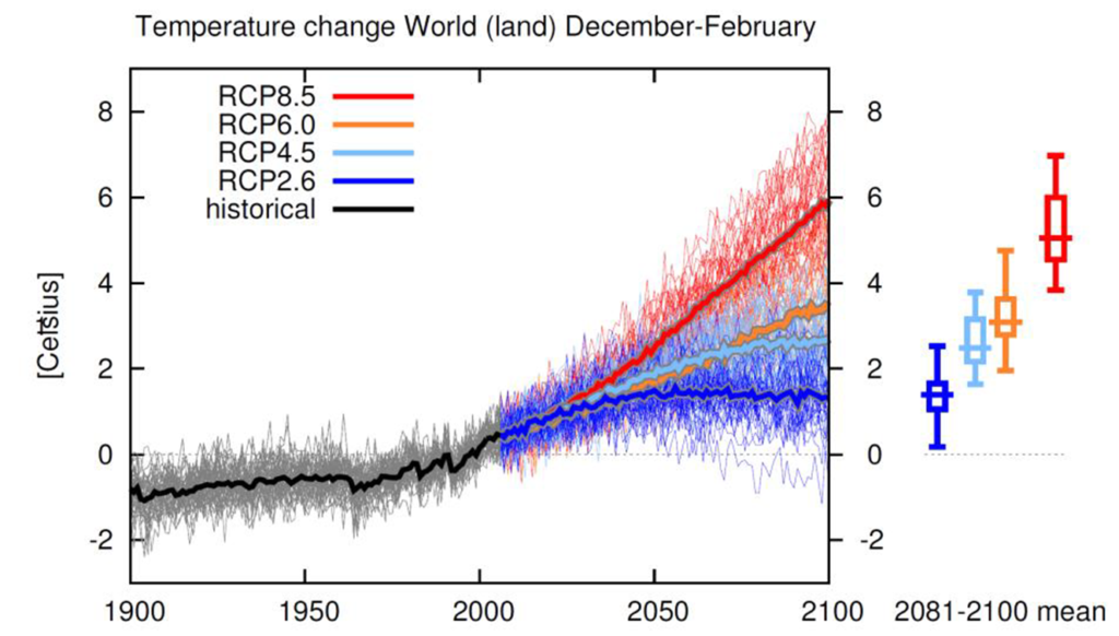
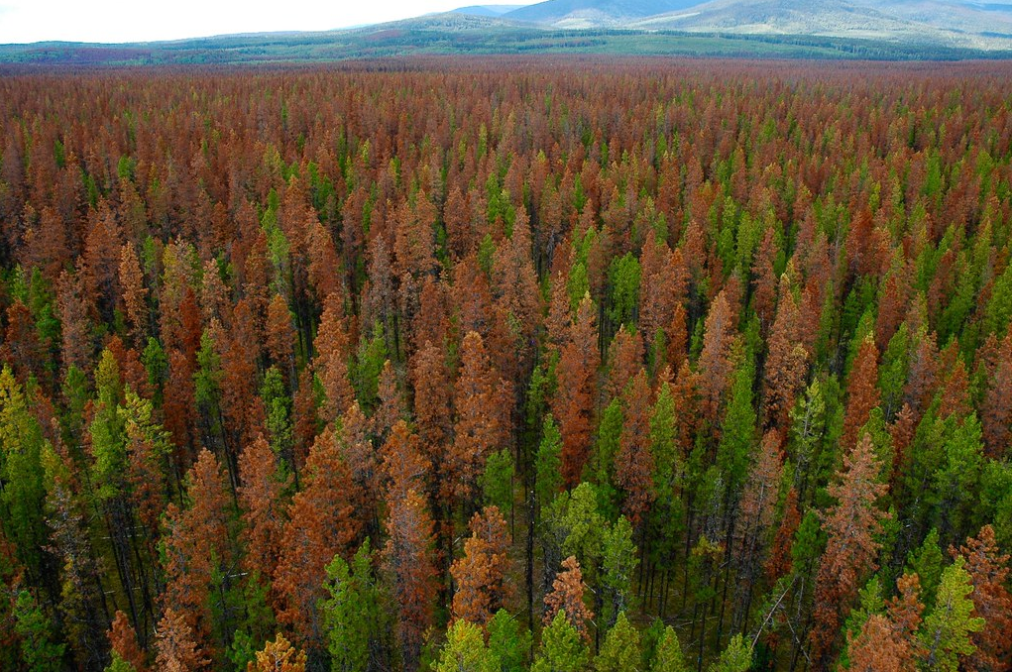
The impacts of climate change on forest ecosystems are likely to compromise tree growth, increase vulnerability to disturbances, and eventually shift in species distributions. Thus, it is likely to require changes in forest planning and natural resource management to mitigate and adapt to climate change. Ecosystem models have widely been used to understand the relationships between ecosystem and environmental conditions, and to provide a “best estimate” about how forests might work in the future and thus guide decision‐making in forest resources management.
An ecosystem model, also called an ecological model, is usually a mathematical representation of an ecological system. It is a simplified form of a highly complex ecosystem in the real world. The ecological system can range in scale from an individual population to an ecological community, or even an entire biome.
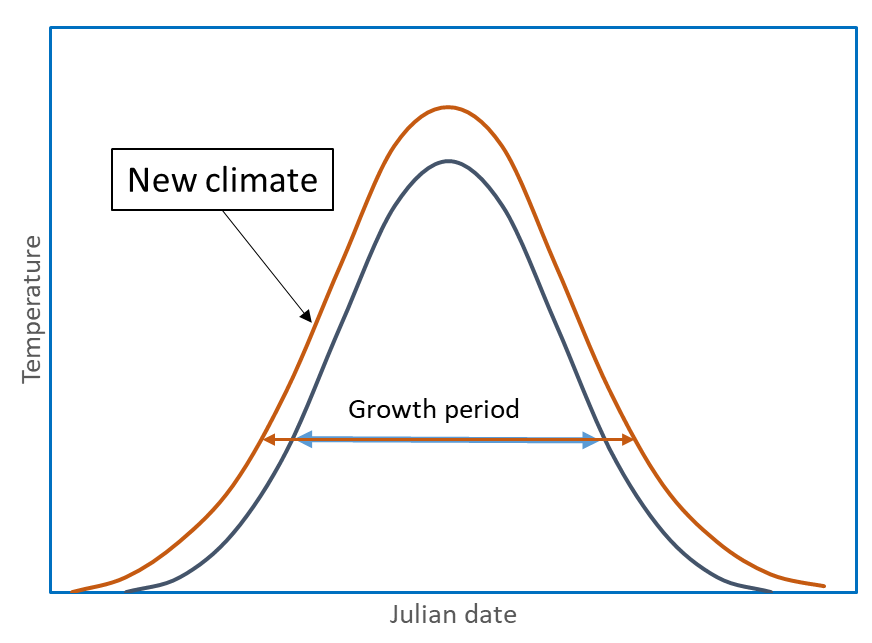
Based on data gathered from the field, ecological relationships—such as the relation of sunlight and water availability to photosynthetic rate, or frost resistance to cold temperature and the length of growth period—are derived, and these are combined to form ecosystem models.
Due to the complexity of ecosystems, it is impossible to capture every possible element of a system in a model. Thus, modelers need to take decisions about which of its features to include and which to disregard. These decisions are usually guided by the aims that the modeler is attempting to achieve. It is desirable to make an ecological model to be general (the model can be applied to a wide range of real-life systems), realistic (the model’s conclusions have a close match to a real-life system) and precise (the model’s predictions for a specific set of circumstances have little or no uncertainty). Trading-off one desideratum in order to achieve greater performance in the other two is often involved in model-building processes.
Ecological models enable researchers to simulate large-scale experiments that would be too costly or unethical to perform on a real ecosystem. They also enable the simulation of ecological processes over very long periods of time (i.e., simulating a process that takes centuries in reality, can be done in a matter of minutes in a computer model). More importantly, ecological models can be used to predict the state of ecosystems under future climates.
Ecosystem models have applications in a wide variety of disciplines, such as natural resource management, ecotoxicology, and environmental health, agriculture, and wildlife conservation. Applications of ecological models in forest resources management to mitigate the negative impact of climate change and help forest trees to adapt to a rapidly changing environment have become particularly important.
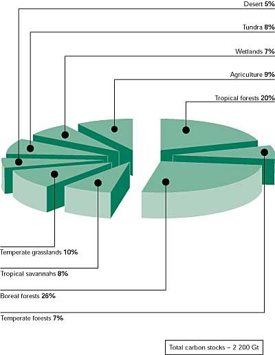
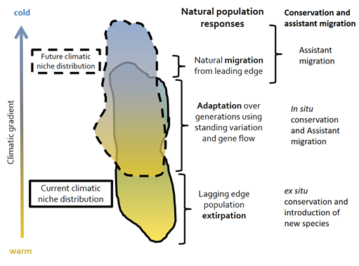
At present, our understanding of the relationships ecosystems and the changing environment is relatively weak.The vulnerability of ecological systems, and the services provided by them, to the impact arising from climate change remain largely unknown. Ecological models have been widely used to assess the impact of climate change in terms of productivity, carbon storage, and vulnerability to disturbances, and to provide information for developing forest adaptive strategies, such as assisted migration at the species level and assisted gene-flow at the population level.
There are two major types of ecological models:
1) Analytic models and
2) Simulation models.
Analytic models are typically relatively simple (often linear) systems, that can be accurately described by a set of mathematical equations whose behavior is well-known. Analytic models are also called correlative models or empirical models.
For example,
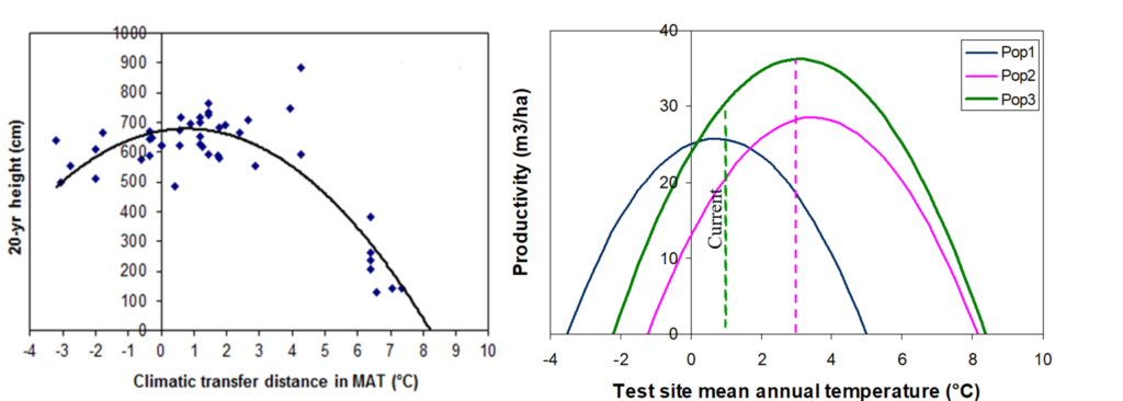
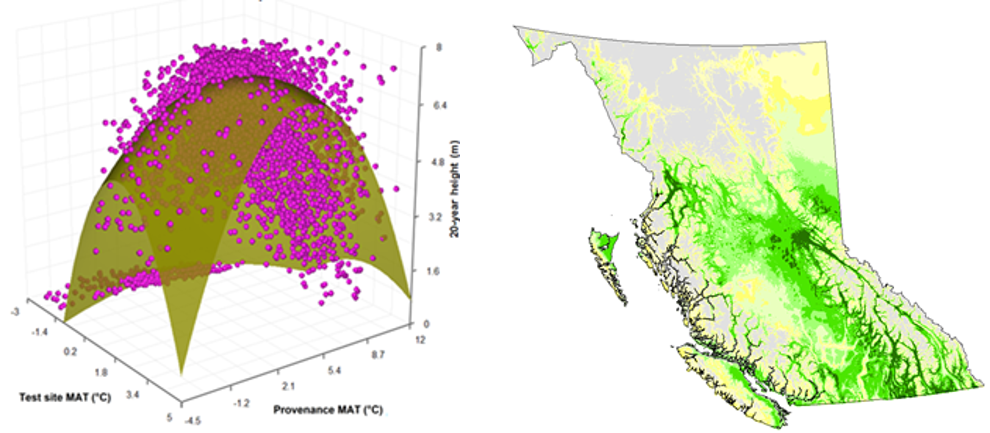
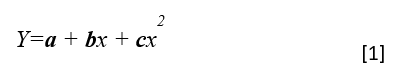
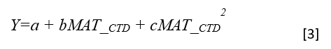
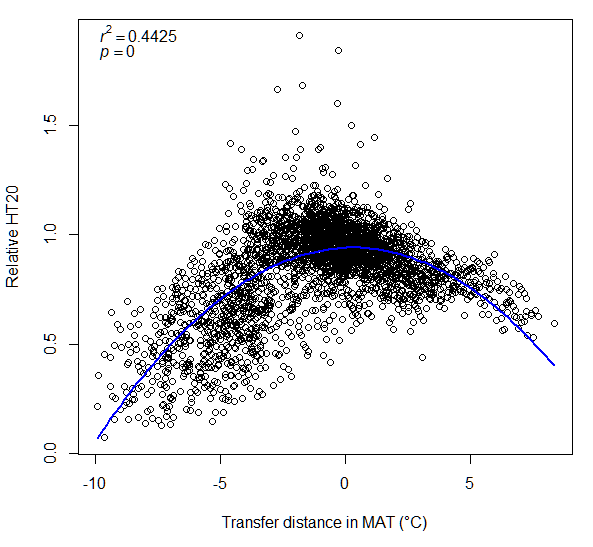
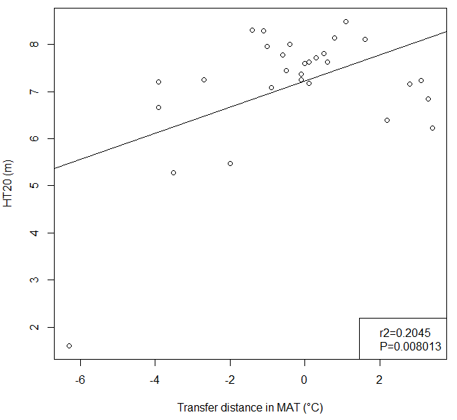
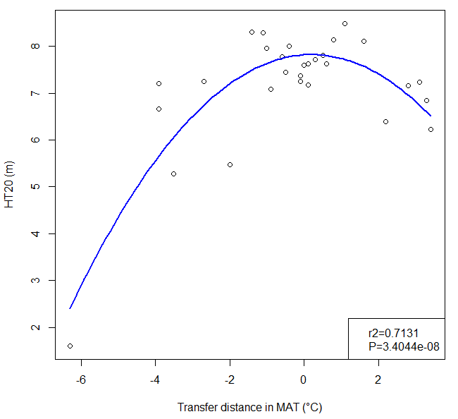
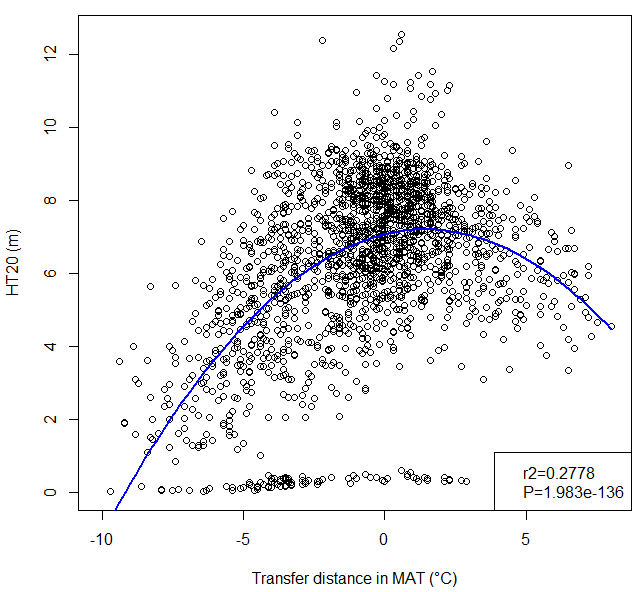
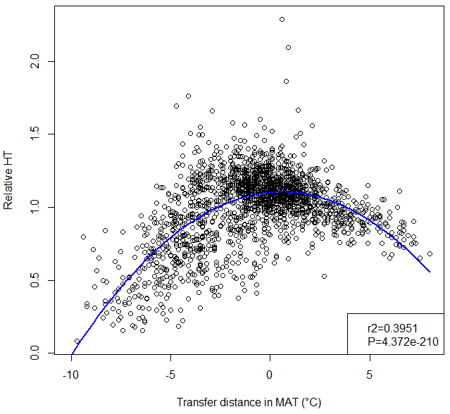
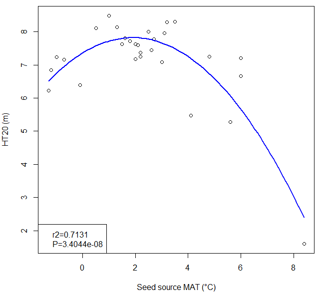
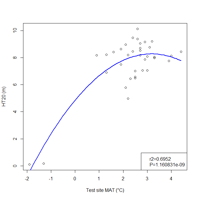
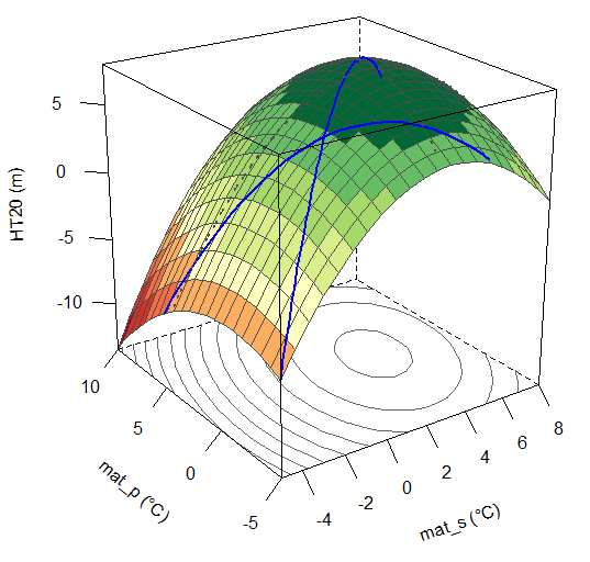
A model of tree height growth of populations originated from different climates that assumes the transfer distance of populations affects the tree height growth in a quadratic relationship as:
Y = b0 + b1 * MAT_td + b2 * MAT_td^2
Where Y is the tree height; MAT_td is the transfer distance in term of mean annual temperature; MAT_td^2 is the quadratic form of the transfer distance; and b0, b1, and b2 are parameters to be determined during the model fitting process.
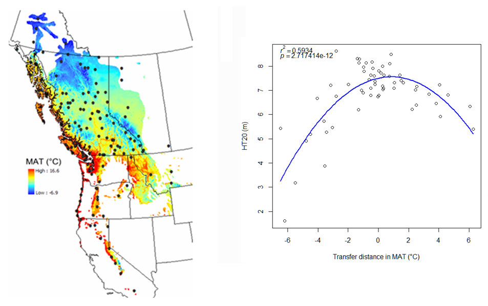
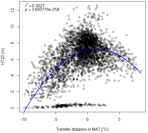
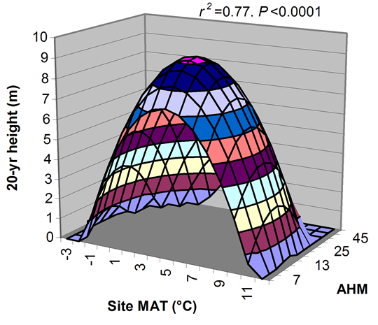
A model can be acceptable if the amount of variance explained by the model is high (or the relationship is strong) based on the statistical significance (P < 0.05), such as the one illustrated in Figure 1.
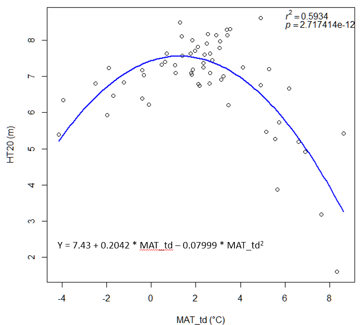
Although the solution to the above simple question is fairly transparent, analytical models describing more complex systems can often become fairly complicated. However, for those comfortable with mathematics, an analytical solution does provide a concise preview of a model’s behavior that is not as readily available with a simulation model. We will focus on this type of models in this course, and more details on analytic or empirical models will come in later lectures.
Simulation models use numerical techniques to solve problems for which analytic models are impractical or impossible. They are also called numerical models or process-based models. A simulation model approach focuses on simulating detailed physical or biological processes that explicitly describe the behavior of a system.
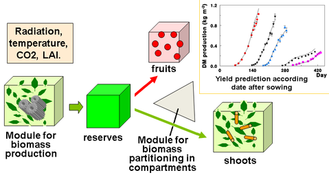
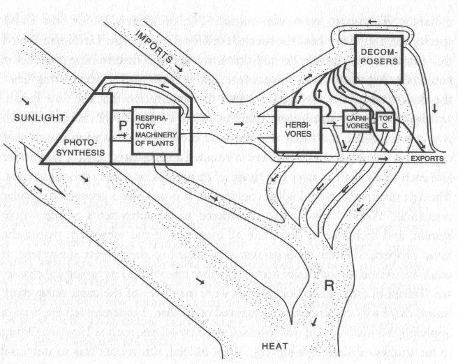
As the name stated, a process-based model can simulate the process or dynamics over time. For example, many process-based models can simulate the tree growth from seedlings to harvest, or simulate the stand performance over rotations.
Both of Empirical and process-based models are applied in modeling the impact of climate change on species distributions, productivity, and vulnerability to stress.
The empirical approach relies on correlative relationships in line with mechanistic understanding, but without fully describing system behaviors and interactions. For example, the model represents the relationship between the transfer distance and tree height of populations. We can see that a strong relationship is represented by the model, but the model does not show the physiological process driving this relationship.
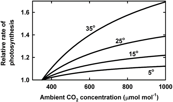
The process-based models, on the other hand, can be more comprehensive and incorporate mechanisms explicitly. For example, many process-based models include the process of how radiation, water, and temperature affect the rate of photosynthesis, and how the biomass generated from the photosynthesis allocates to different parts of the plants, as shown in Figure 2. However, the accuracy of the model predictions is often lower than an empirical model. This is because there are many factors affecting the performance of trees, populations, or an entire ecosystem, and many of them cannot be incorporated into the process-based model.
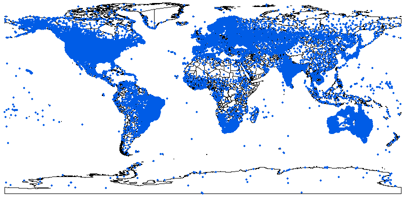
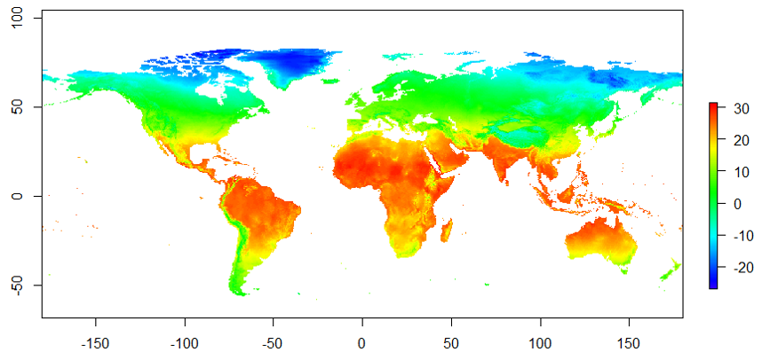
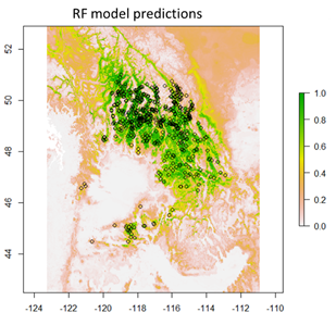
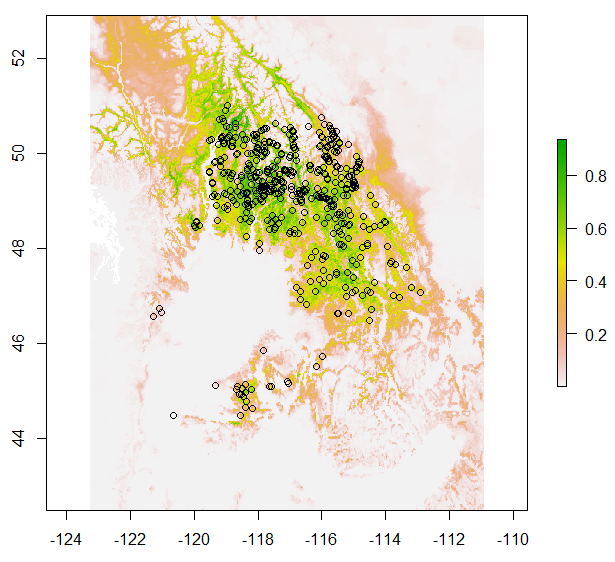
Empirical models based on the occurrence data of a species, particularly with machine-learning algorithms, have demonstrated clear superiority over process-based models in predictions of species distributions. These models are often called species distribution models (SDMs). The occurrence of the species resulted from the process of long-term local adaptation to environmental conditions, interaction with other species, and many other factors. These processes are difficult to model by a process-based model. In contrast, the empirical models do not need to consider these processes, but just relate the occurrence locations with its environmental variables. The relationships are mostly very strong. More detailed comparisons are listed in Table 1.
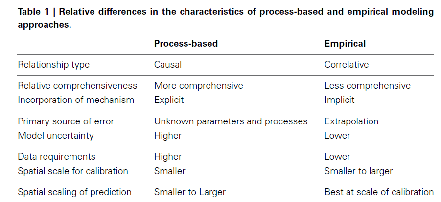
As empirical models are relatively easy to build and will be described in detail in the latter lectures; thus, this section is mostly focused on process-based models.
Ecological systems are composed of an enormous number of biotic and abiotic factors that interact with each other in ways that are often unpredictable, or so complex as to be impossible to incorporate into a computable model.
Because of this complexity, ecosystem models typically simplify the systems to a limited number of components that are well understood and relevant to the problem that the model is intended to solve. Thus, the process of model design needs to begin with a specification of the problem to be solved or the objectives of the model.
The process of simplification typically reduces an ecosystem to a small number of state variables and mathematical functions that describe the nature of the relationships between them. The number of ecosystem components that are incorporated into the model is limited by aggregating similar processes and entities into functional groups that are treated as a unit.
Another important factor in the ecosystem model structure is the representation of the space used. Historically, models have often ignored the confounding issue of space. However, for many ecological problems, spatial dynamics are an important part of the problem, with different spatial environments leading to very different outcomes.
Spatially explicit models (also called “spatially distributed” or “landscape” models) attempt to incorporate a heterogeneous spatial environment into the model. A spatial model is one that has one or more state variables that are a function of space or can be related to other spatial variables.
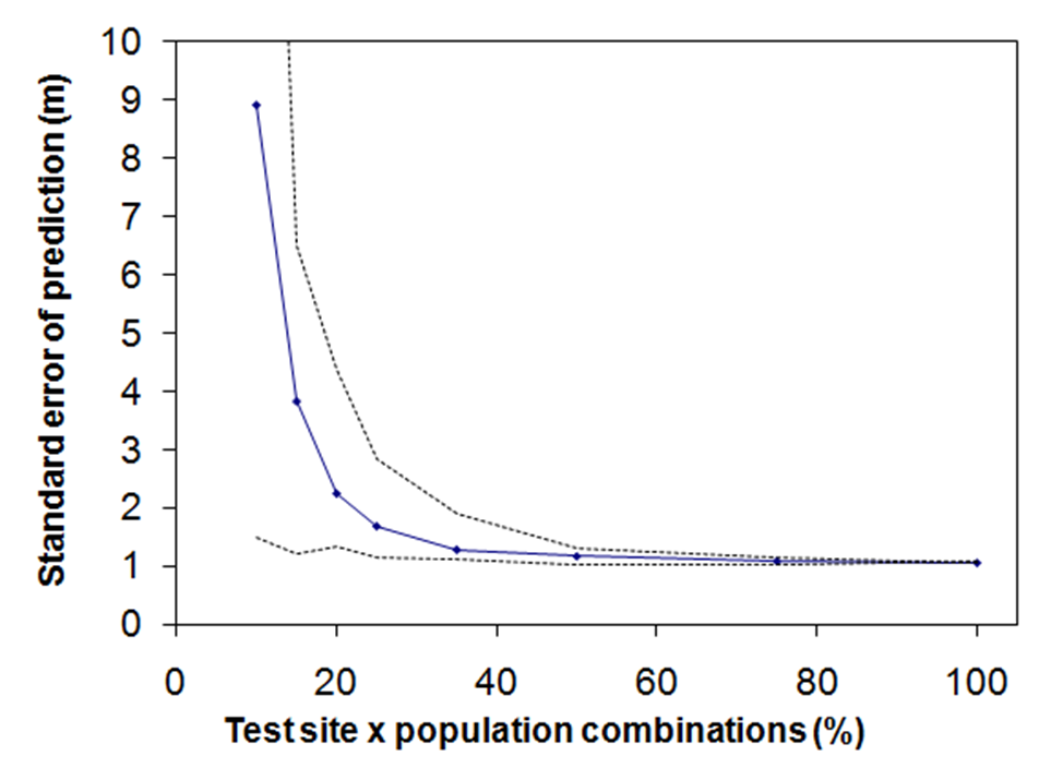
After construction, models are validated to ensure that the results are acceptably accurate or realistic.
One method is to test the model with multiple sets of data that are independent of the actual system being studied. This is important since certain inputs can cause a faulty model to output correct results.
Another method of validation is to compare the model’s output with data collected from field observations.
Model predictions almost always involve errors. Researchers frequently specify beforehand how much of a disparity they are willing to accept between parameters output by a model and those computed from field data.
In process-based models, the environment variables and vegetation are linked up upon the comprehensive physiological processes and functions between them. They often have a high requirement for data input. The process-based approach focuses on simulating detailed physical or biological processes that explicitly describe system behavior. They can be comprehensive and mechanism explicit. All process-based models include some empirical information. Uncertainty in process-based model outputs could be higher than for the empirical approach due to greater model parameters and data inputs to represent the many processes in the system. The application of physiological rules makes process-based models possible to mimic the vegetation growth and display the future species distribution, as well as the forest dynamics.
We will introduce several process-based forest ecological models here.
The 3-PG (Physiological Principles Predicting Growth) forest growth model has been most widely used. The 3-PG model is a simplified physiological processes-based stand growth model developed by Landsberg and Waring in 1997.
A 3-PG model calculates the radiant energy absorbed by forest canopies and converts it into biomass production. The efficiency of radiation conversion is modified by the effects of nutrition, soil drought (the model includes continuous calculation of water balance), atmospheric vapor pressure deficits, and stand age.
3-PG is a deliberate attempt to bridge the gap between conventional empirical growth and yield models, and complex process-based carbon-balance models. It can be applied to plantations, or to even-aged, relatively homogeneous forests. It is a generic stand model, in the sense that its structure is not site or species-specific. However, parameterization is necessary for improving model effectiveness when it is applied for different tree species. The 3-PG model is usually more powerful and effective after the parameter values have been adjusted for aimed tree species.
3-PG consists of five simple sub-models:
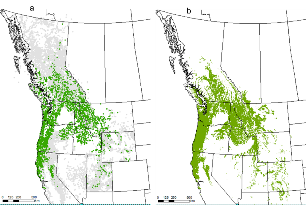
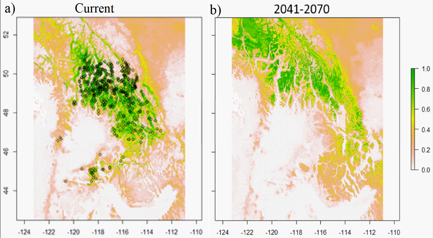
The 3-PG model has been used to stimulate forest dynamic and productivity and estimate future migration direction and distribution under changing climate. A 3-PG model can also be applied together with other tools for a more comprehensive and convincing performance.
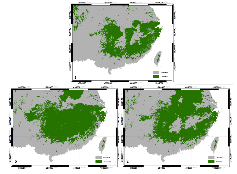
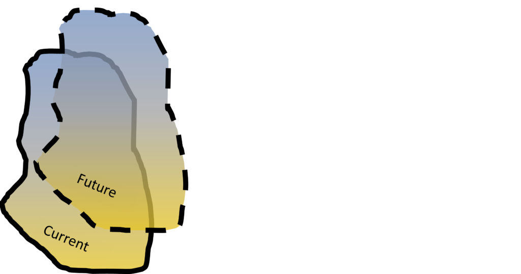
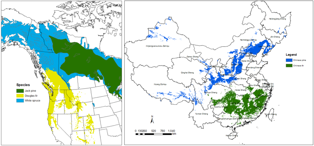
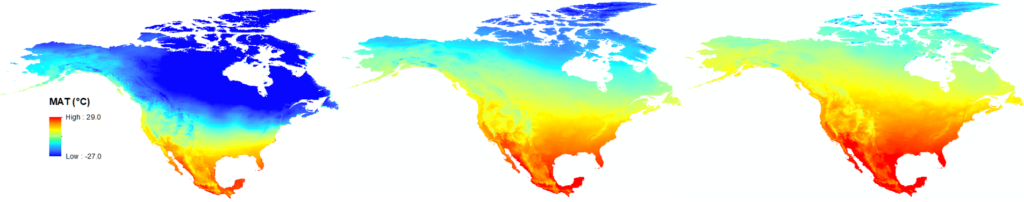
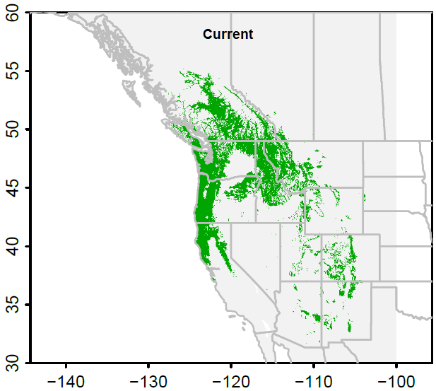
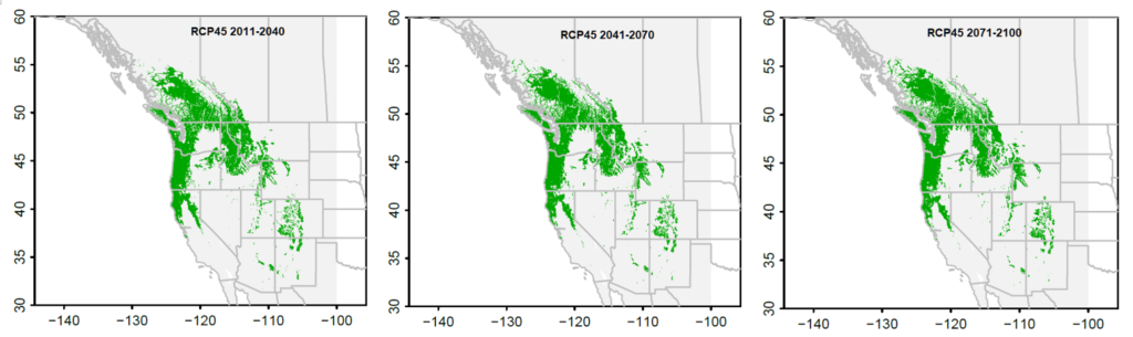
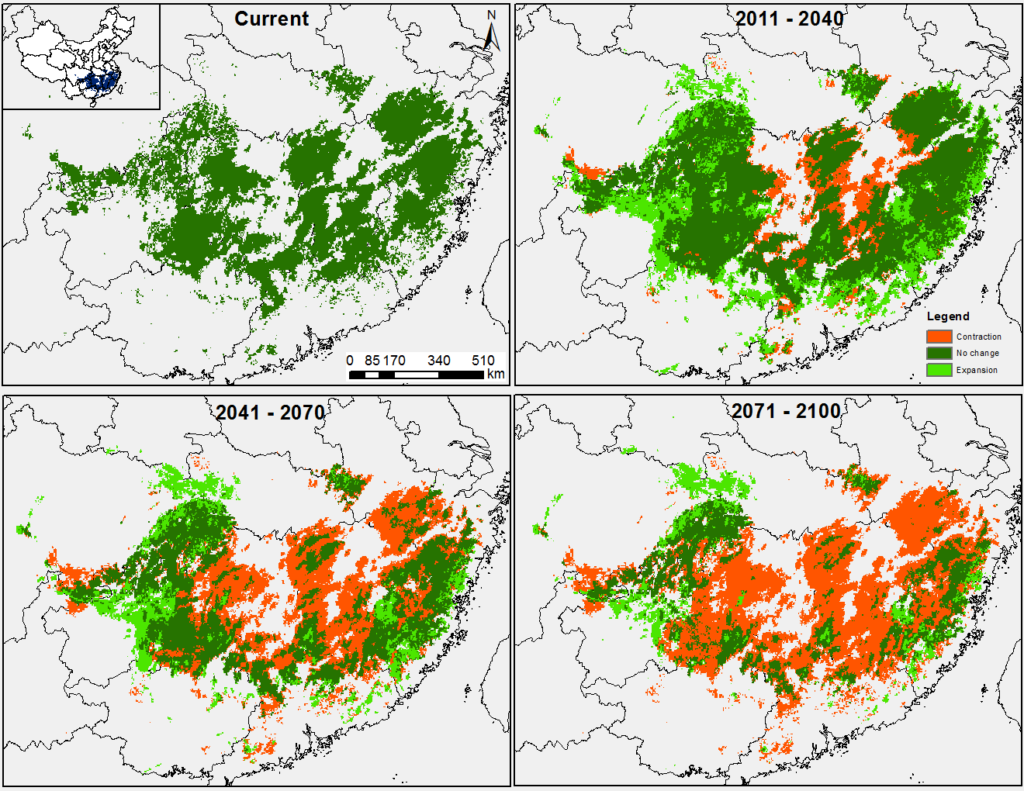
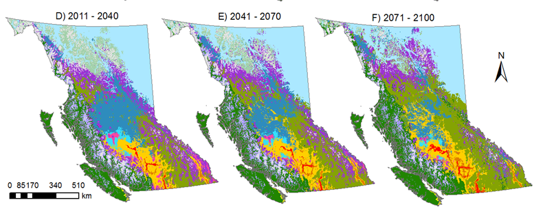
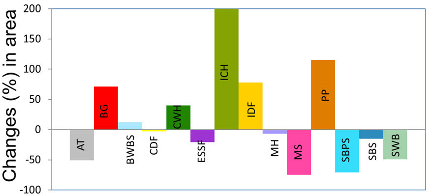
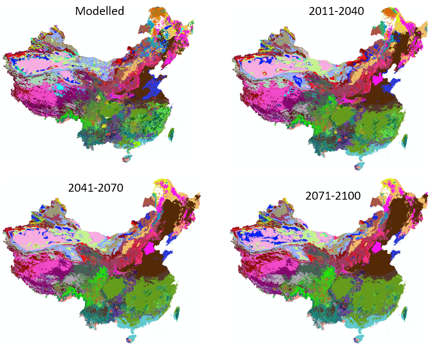
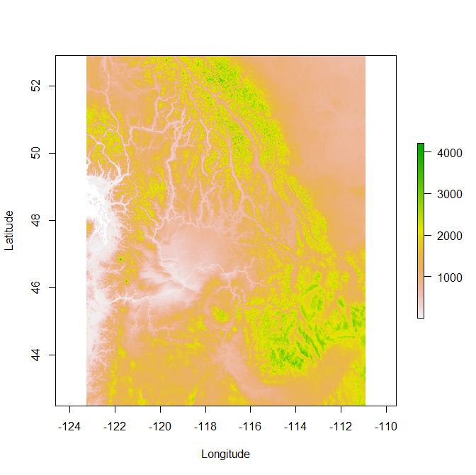
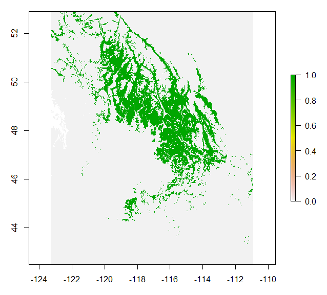
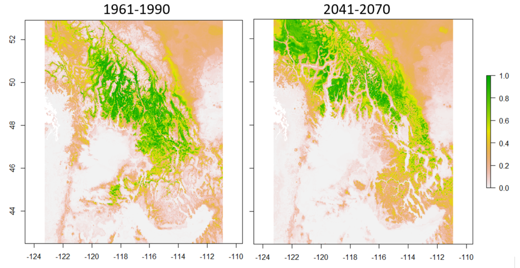
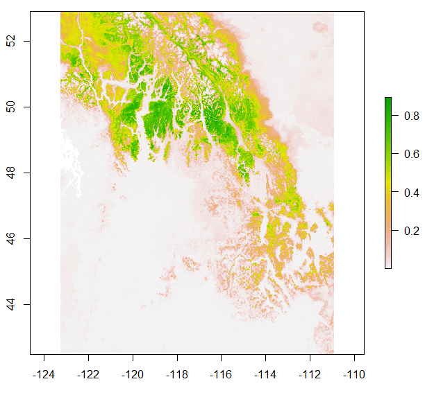
The 3-PG model can be downloaded for free from:
https://3pg.forestry.ubc.ca/software/
FORECAST is a management-oriented, stand-level, forest-growth, and ecosystem-dynamics model. The model was designed to accommodate a wide variety of silvicultural and harvesting systems and natural disturbance events (e.g., fire, wind, insect epidemics) in order to compare and contrast their effect on forest productivity, stand dynamics, and a series of biophysical indicators of non-timber values. The model was developed by Kimmins and his colleagues at the University of British Columbia.
FORECAST can project stand growth and ecosystem dynamics. The projection is based upon a representation of the rates of key ecological processes regulating the availability of, and competition for, light and nutrient resources (a representation of moisture effects on soil processes, plant physiology and growth, and the consequences of moisture competition is being added).
The rates of these processes are calculated from a combination of historical bioassay data (such as biomass accumulation in plant components and changes in stand density over time) and measures of certain ecosystem variables (including decomposition rates, photosynthetic saturation curves, and plant tissue nutrient concentrations) by relating ‘biologically active’ biomass components (foliage and small roots) to calculated values of nutrient uptake, the capture of light energy, and net primary production.
Using this ‘internal calibration’ or hybrid approach, the model generates a suite of growth properties for each tree and understory plant species that is to be represented in a subsequent simulation. These growth properties are used to model growth as a function of resource availability and competition. They include (but are not limited to):
(1) photosynthetic efficiency per unit foliage biomass and its nitrogen content based on relationships between foliage nitrogen, simulated self-shading, and net primary productivity after accounting for litterfall and mortality;
(2) nutrient uptake requirements based on rates of biomass accumulation and literature- or field-based measures of nutrient concentrations in different biomass components on sites of different nutritional quality (i.e. fertility);
(3) light-related measures of the tree and branch mortality derived from stand density and live canopy height input data in combination with simulated vertical light profiles. Light levels at which mortality of branches and individual trees occur are estimated for each species.
The FORECAST model has been widely applied as a long-term management evaluation tool in a variety of forest ecosystems. The FORECAST model simulates the effect of light and nutrient availability on forest productivity but it has no explicit representation of moisture or temperature on ecosystem processes. Thus, the model is not directly driven by climate data. FORECAST Climate has been developed to incorporate these two factors. The foundation for FORECAST Climate was established through the creation of a dynamic linkage with a forest hydrology model including direct feedback to the core processes driving forest ecosystem production.
The Tree and Stand Simulator (TASS) is a biologically based, spatially explicit, individual tree model. By simulating the potential effects of silvicultural decisions and prescriptions, TASS provides yield projections for timber supply reviews and helps resource managers identify investment opportunities. The model is developed and maintained by the Ministry of Forests, Lands, Natural Resource Ministry of Forests, Lands, Natural Resource Operations & Rural Development.
TASS currently exists in 3 main forms:
Photos in Figure 5 show trees remaining after variable retention harvesting by Weyerhaeuser Company Limited (the real world), and the TASS simulations. They are amazingly similar.
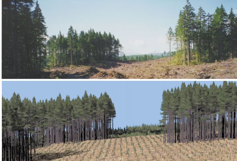
The TASS is a height-driven, biologically oriented, spatially explicit individual tree model (Mitchell 1975). It was designed to produce potential growth and yield tables for even-aged managed stands. It simulates the growth of individual trees in a three-dimensional space with competitions. Tree height, bole diameter, branch length, and crown form and foliage are updated annually. These measures can be affected by inter-tree competition, thinning, pruning, animal damage, site characteristics, defoliation, mortality, and fertilization, as well as genetic variation (or genetic treatments, as shown in Figure 6) in tree growth.
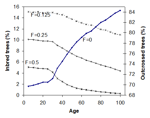
TASS can predict silvicultural treatment response by modelling individual tree crown dynamics and their relationship to bole growth and wood quality. This makes TASS particularly well suited for predicting response to treatments such as
However, effects of climate change have not been incorporated into TASS models. Scientists are working on functions and parameters to link population response to climate into the modeling algorithms.
The software can be download for free at:
The LANDIS-II forest landscape model simulates future forests (both trees and shrubs) at decadal to multi-century time scales and spatial scales spanning hundreds to millions of hectares. The model simulates change as a function of growth and succession and, optionally, as they are influenced by a range of disturbances (e.g., fire, wind, insects), forest management, land-use change. Climate and climate change affect processes throughout the model. LANDIS-II is highly customizable with dozens of libraries (‘extensions’) to choose from.
LANDIS-II is optimized for the simulation of spatial processes and the interactions between spatial processes and patterns. Landscapes within LANDIS-II are represented as a grid of interacting cells with a user-defined spatial resolution (cell size) and extent. Practicable cell sizes can range from a few meters up to a kilometer. All LANDIS models assume that individual cells have homogeneous light environments. Cells are aggregated into ecoregions with homogeneous climate and soils and a user-defined extent, thereby creating a hierarchy of spatial interactions.
The LANDIS-II community is very active with 100s of users and developers worldwide. Everyone is welcome to join the LANDIS-II community and to contribute. All model components are free and open-source. There are active bulletin boards for Users and Developers. And there are meetings and training held every year in various locations across the US and Canada.
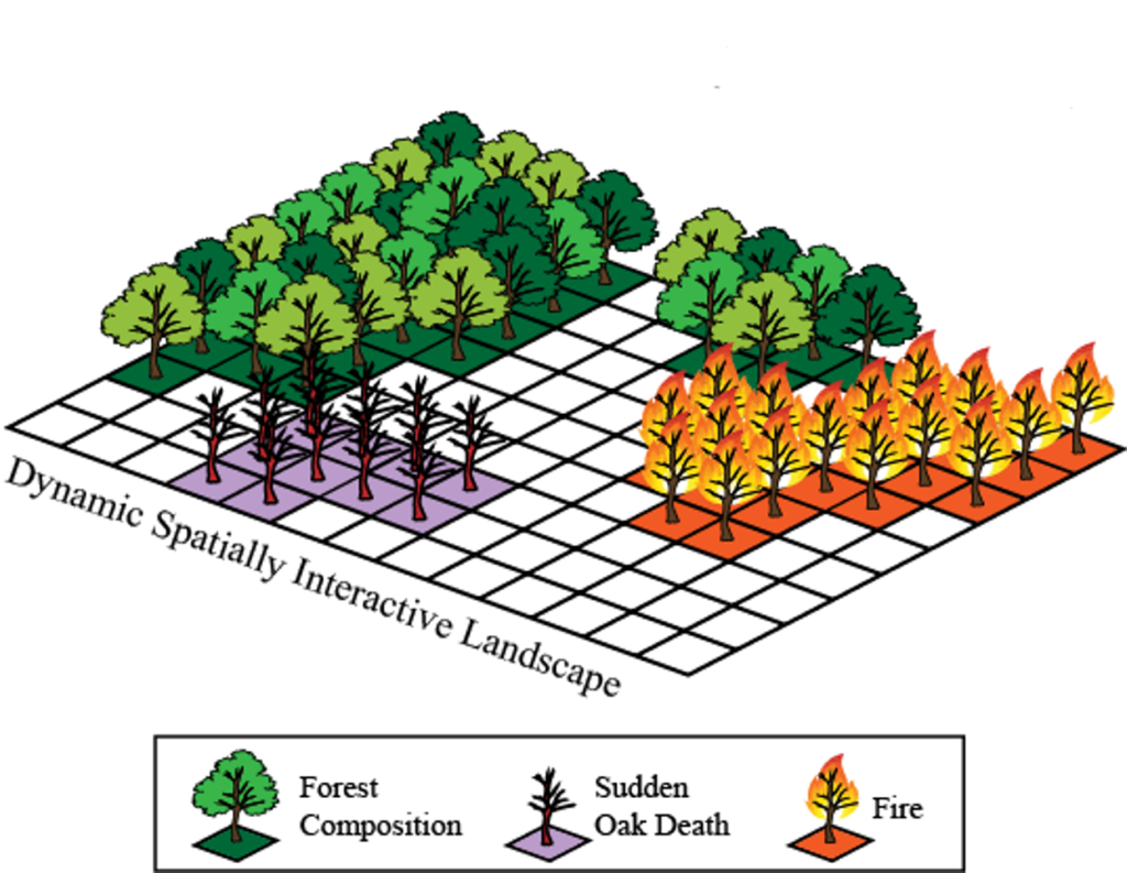
The following video shows an example of Landis II simulations:
The software of the model can be install from: http://www.landis-ii.org/install
By Tongli Wang, Climate Modelling and Forest Applications is licensed under Creative Commons <CC BY-NC-ND 4.0> License
Video #1: Introduction to ClimateNA and ClimateAP – Overview:
A video element has been excluded from this version of the text. You can watch it online here: https://pressbooks.bccampus.ca/climatemodellingforestadaptation/?p=114
Video #2: Introduction to ClimateNA and ClimateAP – How do they work?
A video element has been excluded from this version of the text. You can watch it online here: https://pressbooks.bccampus.ca/climatemodellingforestadaptation/?p=114
Video #3: Introduction to ClimateNA and ClimateAP – Main features:
A video element has been excluded from this version of the text. You can watch it online here: https://pressbooks.bccampus.ca/climatemodellingforestadaptation/?p=114
1. Overview
2. Data sources
2.1. Baseline data
2.2. Historical data
2.3. Future climate data
2.4. Paleoclimate data
3. Dynamic local downscaling
3.1. Baseline data
3.2. Historical and Future climate data
4. Development of additional climate variables
4.1. Calculated climate variables
4.2. Derived climate variables
5. Main features
5.1. Scale-free climate data
5.2. All-in-one package
5.3. Multiple-location and multiple-GCM processing
5.4. Time-series functions
5.5. Map-in and map-out capacity
6. Web versions
7. Spatial data
ClimateNA and ClimateAP are standalone MS Windows software packages that generate scale-free climate data for historical (1901 – 2019), future (2011-2100) and paleo (back to 21,000 years back) periods and years. They also calculate and derive many (>200) monthly, seasonal and annual climate variables to facilitate ecological modeling. Time-series functions are available to generate climate variables for multiple locations and multiple years for historical or future years in a single run.
The scale-free feature allows users to generate climate data for specific locations (instead of grid averages from other climate models) for better accuracy and to generate climate surfaces at any spatial resolution, which is particularly useful for applications at regional and local scales. The scale-free feature is achieved through a dynamic local downscaling to the gridded climate data from PRISM and WorldClim.
The application packages can be downloaded for free. No installation is required. The program can read and output comma-delimitated spreadsheet (CSV) files. The new version of ClimateNA (v6.00) can also directly read digital elevation model (DEM) raster (ASC) files and output climate variables in raster format for mapping. The spatial resolution of the raster files is up to the user’s preference. ClimateNA covers the entire North America (Figures 1).
ClimateAP covers a major part of the Asia Pacific region (Figure 2).
ClimateNA and ClimateAP have been widely in climate change-related studies and applications in almost all fields including forestry, forest genecology, plant ecology, hydrology, meteorology, and agriculture. Currently, there are over 1,500 subscribers and a total of over 1,600 citations.
The monthly baseline data for 1961-1990 normals were compiled from the following sources and unified at 4 x 4 km spatial resolution:
Historical monthly data are developed by ourselves for ClimateNA. For ClimateAP, the historical monthly data are from the Climate Research Unit (CRU ts4.04). Both datasets are provided at the spatial resolution is 0.5 x 0.5° and updated annually.
The climate data for future periods, including the 2020s (2011-2040), 2050s (2041-70), and 2080s (2071-2100), were from General Circulation Models (GCMs) of the Coupled Model Intercomparison Project (CMIP5) included in the IPCC Fifth Assessment Report (IPCC 2014). Fifteen GCMs were selected for three greenhouse gas emission scenarios (RCP2.6, RCP4.5 and RCP8.5) except two GCMs that do not have data for RCP2.6. When multiple ensembles are available for each GCM, an average was taken over the available (up to five) ensembles. Ensembles among the 15 GCMs are also available. Time-series of monthly projections are provided for the years between 2011-2100 for RCP4.5 and RCP8.5 of six GCMs.
ClimateNA (not yet in ClimateAP) contains monthly paleoclimate data were from four GCMs of the CMIP5. The paleo periods covered: 1) Last Millennium or past 1000 years, starting on January 01, 0850; 2) MidHolocene (6,000 years ago); and 3) Last Glacial Maximum (21,000 kyrs ago). Monthly averages were taken over the first 50 years of each period, which is the minimum period available in among the four GCMs.
Instead of using the midpoint values of each grid cell to represent all locations in the grid, ClimateNA and ClimateAP use a combination of bilinear interpolation and local elevation adjustment approaches to downscale the baseline monthly grid data (4 × 4 km) to scale-free point locations. In other words, the programs predict climate data for every specific location.
The program first uses bilinear interpolation to estimate values between midpoints of the four neighbor grids to generate a seamless surface for each monthly climate variables, avoiding step-artifacts at grid boundaries.
The algorithms then retrieve monthly climate data and elevation values for a location from the corresponding grid cell plus eight surrounding cells. The climate and elevation values of the nine cells are used to calculate differences in a climate variable and in elevation between all 36 possible pairs. A simple linear regression of the differences in the climate variable on the difference in elevation is then established, and the slope of the regression is used as the empirical lapse rate for each climate variable at each specific location. The lapse rates are estimated for all the 48 primary monthly variables in ClimateNA and 36 in ClimateAP.
To avoid over-adjustments due to a weak linear relationship, each lapse rate was weighted by the R-square value of the local linear regression. The estimated lapse rate is applied to adjust the bilinearly interpolated values of the location to achieve the downscaling. As the local regressions are dynamically developed along with locations of inquiry, this downscaling method is called a “dynamic local downscaling” approach.
Historical, paleo, and future climate data are first converted to anomalies relative to the reference normal period (1961-1990), bilinearly interpolated, then added onto the downscaled baseline monthly climate normal data (scale-free) to arrive at the final climate surface at a specified resolution or for point data. This approach is called a delta downscaling approach, as illustrated in Figure 5.
With this approach, the original baseline portion (i.e., absolute values for the 1961–1990 normal period) of the historical and future climate data were replaced by the scale-free climate data generated by ClimateNA. Because elevation-adjusted baseline data generated by ClimateNA typically has much higher spatial resolution and accuracy than the historical and future climate data, this process improved the accuracies for both historical and future climate data. However, the approach does not change or improve the anomaly portions of the historical and future climate data except the effect of bilinear interpolation.
The baseline dataset contains 36 primary monthly climate variables, including monthly minimum (Tmin) and maximum (Tmax) temperatures, and monthly total precipitation (Prep). ClimateNA and ClimateAP generate over 200 biologically relevant climate variables to facilitate applications in ecology and forest resource management. Of these climate variables, some are directly calculated from the primary monthly climate variables, and others are derived (or estimated) based on observations from weather stations.
Monthly mean temperatures (Tave) are calculated from monthly Tmin and Tmax. Annual and seasonal mean temperatures and total precipitation are calculated from Tave and Prep, such as mean annual temperature (MAT) and mean annual precipitation (MAP). Other often-used annual climate variables include mean warmest month temperature (MWMT), mean coldest month temperature (MCMT), continentality (TD), which is the difference between MWMT and MCMT, and mean summer precipitation (MSP), ect.. A full list of calculated climate variables can be found at http://climatena.ca/
Many of these additional variables need to be calculated using daily climate data, which are not available in ClimateNA. We estimated these variables based on empirical or mechanistic relationships between these variables calculated using daily observations and monthly climate variables from weather stations from entire North America for ClimateNA, and from the Asia Pacific for ClimateAP. We called these variables “derived climate variables”. These variables were developed at the monthly scale, then summed up to seasonal and annual scales. The steps included: 1) calculating derived climate variables for each month (e.g., degree days) from daily weather station data; 2) building relationships (or functions) between the derived climate variables and observed (or calculated) monthly climate variables; 3) applying the functions in ClimateNA and ClimateAP to estimate derived climate variables using monthly climate variables.
The widely used derived climate variables include growing degree-days (DD>5), cooling degree-days (DD<0), frost-free days (NFFD), frost-free period (FFD), extreme minimum (EMT) and maximum (EXT) temperatures, and climatic moisture deficit (CMD). A full list of derived climate variables can be found at http://climatena.ca/
The derived climate variables are at high accuracies based on the relationships between derived climate variables and monthly temperatures, as shown in Figure 6, for example. Please check Wang et al. (2016) for details.
ClimateNA and ClimateAP generate scale-free climate data that facilitates users to obtain climate data for specific locations, instead of getting grid averages from other data sources. Thus, the scale-free climate data can better reflect the climatic conditions of the locations of interest, as illustrated in Figure 7.
The scale-free feature considerably improves the accuracy of climate variables. For example, ClimateBC (a subset of ClimateNA) predictions of monthly maximum temperatures have much stronger relationships with observations from weather stations (Figure 8).
Scale-free climate data improve the prediction accuracy of ecological models. Climate variables of ecological sample plots predicted by ClimateNA or ClimateAP can better represent climatic conditions of the specific locations of the sample plots, thus can help to build more accurate ecological models. Figure 9 demonstrates an evident improvement in the prediction accuracy of an ecological niche model modeling the biogeoclimatic zones in British Columbia.
ClimateNA and ClimateAP can generate spatial climate data surfaces at any spatial resolution. The output spatial resolution of the climate variables is determined by user’s input dataset. This is particularly important for regional or local applications of ecological models, as a finer spatial resolution is often required to reflect the situation meaningful for practical applications (Figure 10).
ClimateNA and ClimateAP integrate and downscale climate data for historical and Future years and periods. ClimateNA also integrates and downscales climate data for paleo periods (Figure 11). This prevents users from the need to obtain climate data from different sources with different climate variables with different data formats.
ClimateNA and ClimateAP can process an almost unlimited number of locations in a single run. It can also generate climate data for multiple GCMs in a single run.
ClimateNA and ClimateAP can generate time-series climate data for historical (1901-2019) or future years (2011-2100) for multiple locations in a single run. These functions can save users a tremendous amount of time.
Since version 6.0, ClimateNA can read DEM raster file and generate climate variables in raster format for mapping. In previous versions, users need to convert a digital elevation model (DEM) to a spreadsheet file (i.e., a CSV file) as an input file, and also need to convert the output file to raster files. The new versions can directly read a DEM file in raster format and generate climate variables in raster format (as illustrated in Figure 13), which can be directly imported to a mapping software including R.
Web versions of ClimateNA and ClimateAP are available to facilitate easy access to climate data for users dealing with a small number of locations. Users just need to click at the locations on Google Maps to obtain climate variables without the need to type in latitude, longitude, and elevation of the locations as they are automatically retrieved through the Google Map Services. The obtained climate data can be saved to a local computer.
The web versions also allow users to visualize the spatial patterns of major climate variables. Users can use Google Maps’ features to navigate and to zoom in or out around the locations of interest. The maps of the major climate variables can be downloaded in a picture or raster format.
In addition, the web versions serve as a platform to host the spatial data of forest ecosystems and species distributions under current and future climates. This feature has been widely used as a basis for foresters to develop forest adaptive strategies and as demonstrations of the impact of climate change on ecosystems and forest tree species in high school and university classes.
The web version of ClimateNA has two subsets, ClimateBC and ClimateWNA, to focus on regional interests (Figure 14). ClimateBC focuses on British Columbia. In addition to climate data, it hosts forest ecosystems and species distributions. ClimateWNA hosts several major forest tree species in western North America.
The web version of ClimateAP has five subsets, ClimateChina, ClimateLaos, ClimateMalaysia, ClimateMyanmar, and ClimateTaiwan, for different economies (Figure 13). Each hosts climate surfaces and ecosystem projections of its own region.
Pre-generated spatial climate data in raster format for entire North America. The datasets were produced by AdpatWest, which includes climate data for reference and future periods with many GCMs.
By Tongli Wang, Climate Modelling and Forest Applications is licensed under Creative Commons <CC BY-NC-ND 4.0> License
Note: Tutorial videos are embedded within the related content below. Thus, no additional videos are provided here.
1. Download and installation
1.1. Download
1.2. Installation
2. Using the interactive mode
2.1. Coordinates input
2.2. Period selection
2.3. Climate data generating and saving
3. Using multi-location mode
3.1. Input file preparation
3.2. Multi-location processing
4. Multiple GCMs and RCPs processing
5. Generating spatial climate data
5.1. Installing R packages
5.2. Preparing an input file from a DEM file
5.3. Using a DEM as an input file
6. Using time-series functions
6.1. Historical Time Series
6.2. Future time series
6.3. Time-series raster files
7. Using the web version
7.1. Easy access to climate data
7.2. Visualizing spatial climate variables
7.3. Visualizing ecological niche maps of tree species and forest ecotypes
8. Using pre-generated spatial data
ClimateNA and ClimateAP are free for download from their websites at
http://climatena.ca/ and http://web.climateap.net/
By clicking on the interface of each model, you will be led to the downloading page. To download, users are required to register to a mailing list first, which is only for informing new releases and important announcements. After the registration, a downloading link will appear on the page and also be sent to your email. The packages are compressed zip files with sizes of about 600 MB for ClimateNA and 300 MB for ClimateAP.
No installation is required. Users just need to simply unzip all the files and subfolders into a folder on your hard disk and double-click the file ClimateNA _v6.**.exe”. The program does not work on network drives for some unknown reasons.
The exe file can be started even without uncompress the package. However, it does not work properly, and an error message will appear if the “Start” button is clicked.
The program runs on all Windows. It can also run on Linux, Unix and Mac systems with the free software Wine or MacPorts/Wine.
A Youtube video is available to demonstrate the steps of downloading and installation.
Video 1. A tutorial for downloading and installation of ClimateNA (or ClimateAP). Video by Tongli Wang under CC BY 4.0.
The upper section of the interface is for processing single locations. Users need to manually type in the latitude, longitude, and elevation of a location of interest.
The latitude and longitude can be in decimal degrees with the default option. They can also be in degree, minute and second if the “Degree” option is selected. Elevatopm is always in meters. If elevation is missing (or not available), the program still generates climate data based on the bilinearly interpolated elevation values of the baseline dataset, thus, elevation adjustment is not applied in that case.
The default period in both ClimateNA and ClimateAP is the normal period 1961-1990, which is also the period defined as a standard reference period for long-term climate change assessments by the World Meteorological Organization.
More normal period – selection for more normal periods is available by selecting “More Normal Data”. There are nine normal periods available over the period of 1901-2019.
Decadal data – a decadal period can be selected in the same as for selecting a normal period. There are 12 decadal periods available including an incomplete decadal period for the current decade (2011-2018).
Annual data – to generate climate data for a specific year, “Annual Data” needs to be selected in the period dropdown menu. A list of all years will appear for the period of 1901-2019, and an individual year can then be selected.
Future periods – A General Circulation Model (GCM), a Representative Concentration Pathway (RCP), and a future period can be selected under “Future Periods”. There are 15 GCMs for the greenhouse gas emission scenarios RCP4.5 and RCP8.5, and 13 GCMs for RCP2.6. There is also ensemble for each RCP and period over all the GCMs. These ensembles are widely used in climatic and ecological modelling applications.
After a period is selected as mentioned above, it is ready to generate climate data by clicking on the “Start” button. Data generated for annual, seasonal and monthly climate variables are shown in Figure 7. The data values and the coordinates and elevation can be saved as a CSV file by clicking the Save button.
The lower section of the interface of the programs is for processing multiple locations. It requires users to prepare an input file that comprises identifications, latitude, longitude and elevation of the locations of interest. The output file keeps all the columns of the input file, but attach climate variables to each location (or each row). Since version 6.0, ClimateNA can also directly read a digital elevation model (DEM) and generate output files in raster format for mapping. The multi-location mode allows time-series functions to generate climate data for multiple years and processing multiple GCMs, RCPs and periods in a single run.
An input file can be prepared either in Microsoft Excel, a text editor or R. The file must comprise five columns with the first two columns for IDs (e.g., “ID” and “Site” ) and three columns for latitude (lat), longitude (long), elevation (el) as shown in the example below. The columns must be in the same order as shown. If elevation is not available, you have to put in “.” Instead and no elevation adjustment will be applied to that location. No additional columns are allowed. The input file can have almost unlimited number of locations (or rows).
If the file is prepared in Excel, it must be save as a comma-delimited spreadsheet file (a CSV file). If the file is prepared in a text editor, the values must be separated by comma (“,”). If there is a missing value, you need to enter a “.” between two commas. If prepared in R, it need to be save using “write.csv” command.
For making climate maps, an input file can also be converted from a digital elevation model (DEM). This will be explained later in this lecture.
After selecting a period and climate variables, you can select your input file, for example, “Input_test.csv”. Then, click the “Open” button.
The next step is to specify an output file by clicking on the “Specify output file” button. A default output file name is provided, which contains all the information about the input file, period and climate variable category. You may not need to change it in most cases. Then, it is ready to hit the “Start” button to run the process.
A Youtube tutorial shows all the steps and more.
In multi-location mode, climate data can be generated for multiple GCMs, RCPs and periods in a single run. Here are the steps:
All the climate data are generated in one output file. A column is added on the left to show the information of the GCM, RCP and period.
All the steps are also shown in a Youtube:
ClimateNA and ClimateAP can generate spatial climate data at any spatial resolution. A DEM file is required either for preparation of an input file for ClimateAP or directly used as an input file for ClimateNA. The spatial resolution of the DEM file determines the spatial resolution of the output raster files.
We need R to prepare input files and to process output data. Here we will show the steps to install R on Windows, and to install and load R packages. As we will provide the code for each processing work, no programming is required for this lecture. Here are the steps:
1) Download R: https://cran.r-project.org/bin/windows/base/R-4.0.3-win.exe
2) Click to run the exe file “R-4.0.3-win.exe. Follow the instruction on the screen to complete the installation.
3) Click the newly installed R-4.0.3 to start R.
4) Click “File”, then “New script” to open the R code editor
5) Type “install.packages(‘raster’)” and run it by right click and select “Run line or selection”, and follow the instruction on the screen to complete the package installation.
Now you are ready to run the code provided later on.
DEM files can be obtained from various sources. For example, free Digital Elevation Models can be downloaded at https://www.opendem.info/link_dem.html. However, to get a DEM for a specific area is not readily available. The following Youtube tutorial video shows you how.
A simple way to convert a DEM file into an input file for ClimateAP is to do it in R. The following code is used to convert the DEM file “bc80k.asc” in ascii raster format (or “bc80k.tif” in tiff format) to an input file in CSV format (“bc80k.csv”) using raster package (R package can be downloaded at https://www.r-project.org/):
library(raster);
setwd(‘ your working folder‘)
r <- raster(‘bc80k.asc’);
xye <- rasterToPoints(r);
yxe <- cbind(lat=xye[,2],lon=xye[,1],elev=xye[,3]);
yxe2 <- data.frame(ID1=row(xyv)[,1],ID2=row(xyv)[,1],yxe);
write.csv(yxe2,’bc80k.csv’,row.names=F)
A DEM file can be converted into an input file either in ArcGIS Map, Python or other programs as long as the output file meets the requirements as mentioned in 3.1.
ClimateAP or ClimateNA can use this input file to climate data in CSV format as shown in 3.2. To convert the CSV file (e.g., “bc80k_1975Y.csv”) into spatial layers, the following code can be used in R for MAT as an example:
library(raster);
setwd(‘ your working folder‘)
csv <- read.csv(‘bc80k_1975Y.csv’);
MAT <- rasterFromXYZ(csv[,c(4,3,6)]);
plot(MAT)
Since version 6.0, ClimateNA can directly read a DEM raster file as an input file and generate climate variables in raster format for mapping. This makes it much easier to generate spatial climate variables. Here are the steps:
library(raster);
setwd(‘ your working folder‘)
mat <- raster(‘mat.asc’);
plot(mat)
A Youtube video shows the steps:
ClimateNA and ClimateAP can generate time-series climate data for historical (1901-2018) or future years (2011-2100) for multiple locations in a single run. The time-series functions work only for the multi-location process.
Here are the steps to generate historical time-series climate data:
The climate data for all the years involved will be saved in a single CSV file. The information of years is added as the first column to the output file. The size of the file can be huge.
The steps are slightly different for generating time-series data for a future period as it involves selection of GCM, RCP and GCM model runs. Here are the steps:
The two time-series functions also work for generating spatial raster files. The only differences in the steps include:
The following Youtube video shows all the steps mentioned above.
The web versions of ClimateNA and ClimateAP can be accessed at: http://www.climatewna.com/default.aspx
http://climateap.net/default.aspx
Different from the desktop versions, typing in coordinates is optional as they can be automatically obtained by clicking on the Google Map. There are two dropdown boxes for selecting either a historical period or years, or a future period. There are only three GCMs available in contrast to 15 GCMs in the desktop versions. Here are the steps:
Get climate data for other locations or periods by repeating the steps 1) – 4);
7.2. Visualizing spatial climate variables
Several major climate variables are overlaid on the Google Maps and they can be visualized using the Google Map features. When a climate variable is shown, it can be downloaded as a raster file to your local computer by clicking on “Download overlay raster files”.
Ecological niche maps of some major forest tree species are also overlaid onto the Google Maps in ClimateNA and ClimateAP, and their subprograms, such as ClimateBC_Map and ClimateChina.
A large volume of pre-generated spatial climate data using ClimateNA is available for download. However, such spatial data are not available yet for ClimateAP.
Figure 19. Pre-generated spatial climate data in ClimateBC. Image by Tongli Wang under CC BY 4.0.
Steps to download such spatial data are provided at the websites and straightforward. Our next step is to develop an application programming interface (API) based database for spatial climate variables.
By Tongli Wang, Climate Modelling and Forest Applications is licensed under Creative Commons <CC BY-NC-ND 4.0> License
Viedo #1: The concept of ecological niche:
A video element has been excluded from this version of the text. You can watch it online here: https://pressbooks.bccampus.ca/climatemodellingforestadaptation/?p=154
Viedo #2: Impacts of climate change and species occurrence based niche modeling:
A video element has been excluded from this version of the text. You can watch it online here: https://pressbooks.bccampus.ca/climatemodellingforestadaptation/?p=154
Viedo #3: Provenance trials based niche modeling:
A video element has been excluded from this version of the text. You can watch it online here: https://pressbooks.bccampus.ca/climatemodellingforestadaptation/?p=154
1. Adaptation of plant species to climate
2. Ecological niche
2.1. Fundamental niche
2.2. Realized niche
2.3. Niche conservatism
3. Impacts of climate change on ecological niche
3.1. Niche shift
3.2. Mismatch at the population level
4. Climatic niche modeling
4.1. Occurrence data-based modeling
4.2. Provenance trials-based modeling
Of many environmental elements, the climate is the primary factor regulating geographic distributions of plant species. The climate was relatively stable over the last 10,000 years (Figure 1). This period started at around -8500 A. D. after the last Ice Age. This provided an opportunity for plant species to evolve and migrate to geographic locations where climatic conditions are suitable for them to survive, grow and reproduce.
Through long-term evolution and selection, plant species are adapted to a certain range of climatic conditions over the globe. Species that adapted to similar climatic conditions are grouped into biomes (Figure 2). It clearly shows that different climates support different biomes. For example, the tropical climate supports tropical rainforests, while boreal forests distribute in cold climates in the north.
At the species level, each species is adapted to a certain range of climatic conditions (Figure 3). For example, in North America, Douglas-fir is adapted to western North America up to the middle of British Columbia, while spruce and jack pine are distributed further north under a cooler climate. In China, Chinese fir is adapted to a warm and wet climate in the south, while Chinese pine is distributed in the north and northwest adapted to a cool and dry climate.
For a species to maintain its population, its individuals must survive and reproduce. Certain combinations of environmental conditions are necessary for individuals of each species to tolerate the physical environment, obtain energy and nutrients, and avoid predators. The total requirements of a species for all resources and physical conditions determine where it can live and how abundant it can be at any one place within its range. These requirements are termed abstractly the ecological niche.
An ecological niche is originally defined as the position of a species within an ecosystem, describing both the range of conditions necessary for the persistence of the species and its ecological role in the ecosystem. An ecologist, G.E. Hutchinson (1957), suggested that the niche could be modeled as an imaginary space with many dimensions, in which each dimension or axis represents the range of some environmental condition or resource that is required by the species, as illustrated in Figure 4. Hutchinson’s definition of ecological niche formed the basis of niche-based ecological models.
Climate is the most important environmental factor determining species distribution. When only climatic components are considered in studying the ecological niche of a species, the ecological niche is also called a climatic niche. The term climatic niche is widely used in ecological modeling related to climate change.
A fundamental niche is the full range of (physical) environmental conditions that a species can occupy and use, without any other limiting factors present which could constrain the population. In other words, the fundamental niche is the potential niche that the species could occupy if there were no limiting factors. Within its fundamental niche, a species can survive, grow, regenerate and evolve.
A realized niche is the range of conditions actually occupied by a given species. In the real world, a species can only occupy a part of its fundamental niche because of limiting factors, such as competitors, parasites, disease, and physical barriers. Among all the limiting factors, interspecies competition is considered the most important one. Thus, sometimes fundamental niche and realized niche are termed precompetitive and postcompetitive niches, respectively. The difference between a fundamental niche and a realized niche is shown in Figure 5.
The realized niche of a species is reflected by its geographical distribution over the landscape. For example, lodgepole pine is distributed in western North America as shown in Figure 6. Through determining the climatic conditions of the geographic areas occupied by the species, the realized niche for this species can be defined as shown in Figure 7.
Many aspects of the fundamental niche can be conserved over long evolutionary timescales. The tendency of species to retain aspects of their fundamental niche over time is called niche conservatism.
Although debate exists in the literature regarding niche conservatism, the evidence is overwhelming in favor of this theory. Many congeneric plant species in Europe and North America had similar geographic ranges on each continent, a pattern interpreted as evidence for niche conservatism. Niche conservatism is observed in six environmental variables in a sample of more than 1000 species of higher plants in Europe.
Niche conservatism is important because of its relevance to predicting species’ responses to global change. A tendency toward conservatism would mean that species have only a limited capacity to adapt to new environmental conditions.
Climate change is shifting the climatic niche away from the currently occupying geographic locations. Due to the long lifecycle and slow rate of migration of forest trees, such a shift is causing a mismatch between the climate that the species is adapted to and the climate that the species will experience in the future (Figure 8). This is probably the most important challenge for forest species to adapt to a changing climate.
As a result, trees left out of their climate niche will be suffering from sub-optimal climatic conditions and become vulnerable to insects (Figure 9), diseases, and other hazards. This will likely be the case for existing forests in the lagging areas of the species’ climatic niche. Aspen dieback might be an example of the climate niche mismatch (Figure 10).
On the other hand, some areas may become suitable for the species, but it may need a long period for the species to be able to migrate there. Thus, the potential of these areas is not to be used for a long time if we completely rely on the migration of the species on its own.
3.2. Mismatch at the population level
As shown in Figure 11, climatic mismatches occur in two dimensions. One is the mismatch in a climatic niche at the species level (horizontally), and another is the mismatch at the population level (vertically). Due to the geographical shift in the climatic niche, some populations will be left out of the climatic niche of the species as discussed previously. Even for populations that remain within the climate niche, they are no longer under their optimal climate conditions. Survival may not be a problem, but productivity may be compromised. The mismatches in both dimensions need to be considered for developing forest adaptive strategies.
A climatic niche model is to model or define the climatic niche of a given species and to predict its geographic distribution for different climatic conditions, including future climate projections.
4.1. Species occurrence-based modeling
A climatic niche model can be built based on the relationship between the geographical occurrence of a species and its corresponding climatic variables (Figure 12a). Such a model reflects the realized niche of the species (Figure 12b) because the species occurrence is the result of not only the environmental conditions but also migration, local adaptation, and interactions with other species and organisms under recent/historical climatic conditions. The models of this form are typically referred to as climatic niche models, bioclimatic envelope models, or ecological niche models. These terms are often used interchangeably. Occurrence data-based climatic niche models are widely used because the occurrence data is probably the easiest to obtain for a plant species, and models’ prediction accuracies are reasonably high. Species occurrence-based models are analytical models, as discussed previously.
Climatic niche models are widely called correlative species distribution models (SDMs). However, as a climatic niche model defines and predicts the suitable climatic habitat rather than the actual distribution of a species, which involves a series of evolutionary and ecological processes. Therefore, a climatic niche model is, strictly speaking, not a species distribution model (SDM).
A predicted current spatial distribution of the climatic niche may not match well with the current distribution of the species in some areas. Typically, the extent of the climatic niche is greater than the observed range of the distribution. It may not suggest that the model is wrong; instead, it indicates that those areas are potentially suitable for this species to be there. This phenomenon is probably attributable to physical barriers to migration or human disturbances.
4.2. Provenance trials based modeling
Provenance trails in forest trees are traditionally used to determine optimal seed sources for reforestation. Populations collected from a wide range of environments (provenances) are tested in field common-garden experiments under one or multiple planting sites spanning a range of climatic conditions. These materials are now widely used to explore among-population variation along climatic gradients (i.e., genecology functions) and responses of populations to climatic conditions (i.e., response functions). The latter can be used to model the climatic niche at both the population and the species levels.
A response function can be developed for an individual population. Response functions are used to predict the response of adaptive traits including growth and survival to climate. The range of the climatic conditions suitable for the population can be used to define the climatic niche of the population. When individual response functions are integrated, it can be used to model the climatic niche of the species.
Since the trees growing in the common-garden experiments are free from interspecific competitions and the limit of migration, the climatic niche predicted by a response function can be considered as the fundamental niche of the population or the species. This will be discussed in detail later.
By Tongli Wang, Climate Modelling and Forest Applications is licensed under Creative Commons <CC BY-NC-ND 4.0> License
Video #1 and #2: Concept of genecology
A video element has been excluded from this version of the text. You can watch it online here: https://pressbooks.bccampus.ca/climatemodellingforestadaptation/?p=173
Video #3: Transfer functions:
A video element has been excluded from this version of the text. You can watch it online here: https://pressbooks.bccampus.ca/climatemodellingforestadaptation/?p=173
Video #4: Genecology functions and predictors:
A video element has been excluded from this version of the text. You can watch it online here: https://pressbooks.bccampus.ca/climatemodellingforestadaptation/?p=173
1. Overview
2. Definition of genecology
2.1. Definition
2.2. Some relevant terms
2.3. Objectives of genecology
3. Transfer functions
3.1. Provenance test
3.2. Transfer functions
3.3. Features and limitations
4. General transfer functions
4.1. General transfer functions
4.2. Relative performance-based general transfer functions
4.3. Limitations of general transfer functions
4.4. Universal transfer functions
5. Genecology functions
5.1. Genecology functions
5.2. The difference in genecology functions among environments
6. Geographic vs. climatic variables
6.1. Representation of environmental variables
6.2. Accessibility
6.3 local vs. universal
6.4. Applicability for climate change
6.5. Non-climatic factors
As mentioned in the previous topic and shown in Figure 1, climatic mismatches occur in two dimensions. One is the mismatch in the climatic niche at the species level (horizontally), and another is the mismatch at the population level (vertically). The niche-based models at the species level can be used to predict the shift in the climatic niche at the species level. Genecology functions are to predict among-population variations within a species.
Genecology is the study of intraspecific genetic variation in relation to environmental conditions. In other words, it is to study the relationships between genetic variation and environmental gradients within a species.
Genecology is often referred to as ecological genetics, which is actually more widely used. However, strictly speaking, ecological genetics is the study of how ecologically relevant traits evolve in natural populations, which covers inter-species interactions. Nevertheless, these two terms are used interchangeably.
Provenance – the place of seed origin (or seed source).
Population – a group of individuals of the same species that live in a particular geographical area, and have the capability of interbreeding. Individuals from the same provenance is called a population.
Provenance is often used to refer a population although it is not accurate. Thus, provenance and population are often interchangeably in genecology.
Provenance test (or provenance trial) – a common garden experiment that compares trees or plants collected from different provenances. Typically provenance tests compare widely separated seed sources. The test may contain multiple test sites.
Genetic variation – can be defined at the individual level as the difference in DNA among individuals, or at the population level as among-population variation due to difference in allele frequency.
Genetic cline – a geographic or climatic pattern of change in a trait.
Genetic and environment interaction (GxE) – different genotypes respond to environmental variation in different ways.
Operational objectives:
Theoretical objectives:
Transfer functions are most commonly used in genecology to reflect the effect of transfer distance of populations in terms of geographical or climatic variables. A provenance test is required for developing a transfer function.
Figure 2 shows a typical provenance test. Populations from 140 provenances range-wide were planted in 60 common garden trials (planting sites) in British Columbia (BC), Canada. At each site, an incomplete block design was used to include 60 populations due to a large number of populations. Thus, not every population was tested at all the 60 sites except seven reference populations. Tree height was measured at age 20.
As illustrated in Figure 3, populations are transferred from their origins to a test site in the mid of BC in the provenance test. Those populations grow under new environmental conditions, and their performances may be affected. As the populations are grown under the same climatic conditions (at the same test site), the difference in the performance of populations is supposed to be due to genetic variation among the populations.
The genetic variation observed in a provenance trial at each test site may be associated with the population transfer distance. It is hypothesized that the longer the transfer distance, the larger the transfer effect. Thus, the transfer distance is used as a predictor in a transfer function as:
Where, Y is the performance of a population; x is the transfer distance; and a, b, and c are parameters to be estimated to fit the model.
The transfer distance can be in a physical distance for geographical variables (e.g., latitude, longitude, or elevation), or in units for climatic variables (e.g., temperature and precipitation). Climatic variables are increasingly used as they have many advantages over geographical variables, particularly for predicting the impact of climate change on forests.
Climatic variables are needed for all the provenances to build a transfer function using the transfer distance in climatic variables, as shown in Figure 4. A map of mean annual temperature (MAT) covering the lodgepole pine distribution and a transfer function for a test in the mid of BC.
The transfer distance in MAT (MAT_CTD) is calculated as:
MAT_CTD = MAT_s – MAT_p [2]
Where, MAT_s is the MAT of the test site, MAT_p is the MAT of the provenance. Then, the transfer function is written as:
Populations with negative transfer distances on the left of the plot were transferred northward (from warmer climates to cooler climates). On the other hand, populations with positive transfer distances on the right of the plot were transferred southward (from cooler climates to warmer climates). Populations with zero and around zero transfer distance are considered local populations. The local populations have the best performance; however, the peak of the curve is not always exactly at the zero transfer distance point, as shown in Figure 4.
A transfer function represents the transfer effect of populations. It reflects the genetic effect of climate on populations. It is intuitive and easy to build. However, there are several limitations for transfer functions. A transfer function built for one site may be different from the one built for another site, even with the same group of populations. Thus, a transfer function developed for one site, strictly speaking, only represents the transfer effect of populations under the particular environment of that test site. The number of test sites is limited for most tree species, and people tend to oversell the results drawn from these sites. Therefore, we need to be aware of such a risk of using a transfer function built for one environment to represent the situations for other environments.
Due to the limitation of transfer functions discussed above, general transfer functions were proposed. The only difference between a transfer function and a general transfer function is that data from all test sites are pooled together in developing a general transfer function. The formulas [1] – [3] all apply to a general transfer function.
The curve of a general transfer function shown in Figure 5 was developed based on the observations from the same provenance test mentioned above. The relationship between the performance and transfer distance of populations in a transfer function is usually weak.
The most important reason for a general transfer function being weak is the difference in the performance of populations among sites. For example, the outliers at the bottom of Figure 5 are populations growing at several cold sites in the north. Their total height at age 20 is less than a meter. An approach was developed to overcome this problem by using relative performance. With this approach, the performances of populations are converted to proportions relative to the performance of the local population. It can substantially improve the relationship of the general transfer function, as shown in Figure 6. It worths of reminding that the relative performance needs to be converted back to actual performance in applications of this model.
In addition to the weak relationships of general transfer functions as mentioned above, there are other limitations for general transfer functions. As discussed earlier, the transfer effects of populations are different among test sites. By pooling the data across all test sites to develop a general transfer function, the difference in the transfer effect of populations among test sites is averaged out, as illustrated in Figure 7. This compromises the prediction power of general transfer functions. In addition, the same amount of transfer distance may have different transfer effects. For example, for a -2°C transfer distance in temperature, the transfer from 2°C to 0°C may be different from the transfer from 10°C to 8°C. This point will be further discussed later in comparison with genecology functions. Nevertheless, general transfer functions are the simplest to implement; thus it is still commonly used.
Where,
X is transfer distance;
P is provenance climate;
XP is the interaction term;
rs are some random effect terms.
The universal transfer function can overcome the problems listed above, but the random terms cause additional problems. The model is too complicated and often fail to converge. It used only one climate variable in applications so far, which can compromise the model capability.
.
A genecology function uses the environmental variables of provenances, rather than transfer distance used in both transfer functions and general transfer functions. Thus, a genecology function represents the relationship between the performance of populations and environmental variables of the population origins (or provenances), which exactly reflects the definition of genecology. A genecology function can be written as:
Y=a + bx + cx2
Where, Y is the performance of a population; x is an environmental variable of provenance; and a, b, and c are parameters to be estimated to fit the model.
Using the same data for building a transfer function in Figure 4, a genecology function is developed, as shown in Figure 8. Although the shapes of the curves are quite different, the R square values are identical between the two functions.
Genecology functions developed for different environments show different relationships (Figure 9). Thus, a genecology function built based on information from one environment may not represent the relationship for other environments. This is the same as for the transfer function.
6. Geographic vs. climatic variables
Both transfer functions and genecology functions can be built with either geographic or climatic variables. There are advantages and disadvantages to use geographic or climatic variables as predictors. We will make a detailed comparison between the two.
Geographic variables are not direct environmental variables, whereas climatic variables are. However, geographic variables are related to environmental variables. For example, elevation is strongly related to temperature, which affects plant performance, as illustrated in Figure 10. Thus, they are often used to substitute environmental variables. However, if we build a greenhouse at the top of the mountain, we can grow any plant that can only grow at the bottom of the valley. It suggests elevation itself does not affect plant growth.
Geographic variables are more accessible than climatic variables. That is why they were more often used for experimental design and data analysis in the past. With increasingly available climate data, accessing climatic variables are becoming as easy as accessing geographic variables. Especially with the scale-free climate models ClimateNA and ClimateAP, climatic variables can be easily obtained for any specific location within their coverage.
A transfer function or a genecology function built with geographic variables only works for the region where the model is built. This is because of the effect of a geographic variable changes from region to region, or location to location. For example, 2000 m in elevation in California is suitable for many plants to growth; but the same elevation in BC is beyond the treeline. Also, an increase in elevation by 100 m in California will result in a decrease in temperature by 0.65°C; but the same change in northern BC will only result in a decrease in temperature by about 0.2°C. In contrast, a transfer function or a genecology function built with climatic variables can be applied anywhere.
A transfer function or a genecology function built with geographic variables cannot be used for assessing the impact of climate change as geographic variables are static and have no future projections. In contrast, climatic variable based functions can predict the past and future. That is the reason why genecology has been a hot area.
Geographic variables are still useful to reflect some important non-climatic factors. Genetic variations among populations are also affected by spatial autocorrelation involving migration and gene flow related to physical barriers and distance. Those factors sometimes need to be included in genecology functions. We will discuss this further in the next topic.
By Tongli Wang, Climate Modelling and Forest Applications is licensed under Creative Commons <CC BY-NC-ND 4.0> License
Lecture videos:
A video element has been excluded from this version of the text. You can watch it online here: https://pressbooks.bccampus.ca/climatemodellingforestadaptation/?p=188
1. Overview
2. Definition
3. Response functions with a single variable
3.1. Objectives
3.2. Provenance test and climate data
3.3. Finding populations for future climates
3.4. Anchor points
4. Response functions with multiple climatic variables
4.1. Function
4.2. Response surface and function parameters
4.3. Model interpretation
5. Multiple response functions
5.1. Objectives
5.2. Putting multiple response curves on the same plot
5.3. Comparisons among multiple response curves
5.4. Limitations
6. Universal response functions
6.1. Objectives
6.2. Function
6.3. Features
The concept of the population response function is relatively new in ecology. It was first introduced to model forest trees by Dr. Rehfeldt in 1999. It can predict the mismatch at the population level individually (vertically in Figure 1). It can also predict the mismatch at the species level integratively if an adequate number of populations are modeled (both vertically and horizontally in Figure 1). In addition, the climatic niche model by using response functions represents the fundamental niche of the species instead of the realized niche as modeled using presence-absence data.
A population response function describes the response of a population to the change of environmental conditions. It represents the environmental effect on the population. It also reflects the plasticity of the population over a range of environmental conditions.
This is contrasting to genecology functions or transfer functions, which are to model among-population variations in performance along environmental gradients of population origins. They reflect genetic variation in populations associated with environmental factors. A common feature of these two kinds of models is that they both are built based on provenance tests.
A typical linear and quadratic population response functions can be written as:
Y = a + bx [1]
Y = a + bx + cx2 [2]
Where, Y is the performance of a population; x is one (or more) environmental variable of test sites; and a, b, and c are parameters to be estimated to fit the model.
Similar to a genecology function, a response function can be with geographical variables (e.g., latitude, longitude, or elevation), or climatic variables (e.g., temperature and precipitation). Climatic variables are increasingly used as they have many advantages over geographical variables, particularly for predicting the impact of climate change on forests. Up to date, all response functions are built with climatic variables.
A single climatic variable often plays a dominant role in affecting the performance of populations. For simplicity, we can build a response function with just one climatic variable. With a single climatic variable, a response function can reflect a simple linear relationship with a single climatic variable. It can also be built with a polynomial function, such as a quadratic, a cubic function. A quadratic function showing a bell-shape response curve is most commonly used as most climatic variables have an optimal range suitable for a plant species to grow.
Let’s use the same provenance test shown in Figure 2 to demonstrate response functions. In the provenance test, each population was planted at multiple test sites. After 20 years of growth under different environmental conditions, the population showed substantial differences in performance among the test sites.
After we obtained climate data from ClimateNA, we can develop a response function for this population to represent the effect of temperature on the tree height of the population. As shown in Figure 3, the response function predicts the performance of the population Pop1 in different temperatures with its optimal performance around its local temperature. With an increase in temperature by 2°C due to climate change, the predicted productivity is predicted to drop substantially. We need to find populations that perform better in a warmer climate. Ideally, we may found populations that can perform well over a broader range of temperatures covering both the current and future climates.
Most provenance tests have a limited number of test sites due to the high cost and availability of planting sites. Also, due to a large number of provenances, there is no enough space to include all provenances. As a result of these situations, some provenances are often not tested at some extreme climatic conditions and make it is difficult to build an effective response function. For the latter case, a genecology function can be used to predict the performance of the missing populations at the site where the genecology function is built for. The predicted values are called anchor points as they play a role to anchor the curve down at the end of the species range. Details are described in Wang et al. (2006).
A single variable is often not sufficient to explain the variation in the performance of a population across different environmental conditions. In those cases, two or more environmental variables are needed to be included in the model to increase its explanatory power. Then, the formula of a quadratic response function with multiple variables becomes:
Y = b0 + b1x1 + b2cx12 + b3x2 + b4cx22 + …
Where, Y is the performance of a population; x1, x2, …, are the climatic variables; and b0, b1, b2, …, are parameters to be estimated to fit the model.
We use the dataset from the same provenance test for lodgepole pine to illustrate the response surface. A quadratic response function is built with two climatic variables, mean annual temperature (MAT) and annual heat-moisture index (AHM), as predictors. The response surface represents the response function is shown in Figure 4. The parameters estimated for the response function and the significance of the predictors are listed in Table 1.
Tabe 1. Parameters estimated and significance of the predictors
Estimate | Std. Error | t value | Pr(>|t|) | Significance | |
(Intercept) | 1.731036 | 1.758753 | 0.984 | 0.3298 | |
MAT | 2.231324 | 0.511851 | 4.359 | 6.68E-05 | *** |
AHM | 0.303606 | 0.145037 | 2.093 | 0.0415 | * |
MAT^2 | -0.24298 | 0.05008 | -4.852 | 1.28E-05 | *** |
AHM^2 | -0.00755 | 0.003411 | -2.214 | 0.0315 | * |
MAT*AHM | -0.0126 | 0.028548 | -0.441 | 0.6608 |
The information from the response surface shown in Figure 4 and the parameters estimated in Table 1 shows that MAT plays a dominant role in affecting the performance of the population, while AHM also significantly contributes to the model. However, the interaction between MAT and AHM does not significantly contribute to the model. In total, the model explains 77% of the total variation in tree height of the population among all the test sites. The model is highly accurate at P < 0.0001.
The response surface also shows: 1) this population can grow within the range between -3°C and 11°C for MAT and between 5 and 45 for AHM, but slightly varying depending on each other (i.e., climatic niche of this population); 2) the optimal climatic condition for this population is a combination between MAT at around 5°C and AHM at about 13; however, 3) the population can grow well between 3°C and 7°C for MAT and between 10 and 20 for AHM.
A population response function built for a population reflects the characteristics of the given population. In other words, the function does not represent the responsive nature of other populations. To understand the difference among populations in this regard, we need to build response functions for other populations individually and then make comparisons among them. If there are a sufficient number of populations having response functions built, they can provide an overview of the response to climate at the species level.
After response functions are built for multiple populations, to make comparisons among the response functions is important. Putting the response curves on the same plot is the most straightforward approach to make such a comparison. However, it is difficult to do so if the response functions are built with two or more climate variables. A solution for this is only to compare the response against the dominant variable while keeping the other variables constant or at their optimums. Figure 5 shows multiple response curves against MAT on the same plot while keeping AHM at its optimum for lodgepole pine.
Figure 5. Comparisons in response curves among populations of lodgepole pine in BC. Image by Tongli Wang under CC BY 4.0.
Through comparisons among the response curves shown in Figure 5, the following results can be drawn:
These results drawn from the comparison provide a scientific basis for developing adaptive forest management strategies.
Response functions predict the response of populations to the change in environmental conditions, primarily climatic conditions. It is probably the most straightforward approach for understanding the impact of climate change on the performance of populations and for developing forest adaptive strategies. However, it has the following two limitations:
Genecology functions and transfer functions represent variation in the performance of populations caused by their origin (genetic effect). In contrast, response functions explain the variation in performance in response to differences in climatic conditions among test sites (environmental effect). Both have limitations in practice applications; a genecology function or a transfer function built for a test site may not apply to other environments. Similarly, a response function developed for a population may not apply to other populations. A universal response function is developed by Wang et al. (2010) to overcome these limitations by integrating both the genetic effect and the environmental effect into one model, as illustrated in Figure 6.
Figure 6. Illustration of integrating genecology functions and response functions to build a universal response function.
A universal response function is a combination of a genecology function and a response function. A genecology function can be written as
Y = b0 + b1x1 + b2x12
Where, Y is the performance of a population; x1 is one (or more) environmental variables of provenance; and b0, b1, and b2 are parameters to be estimated to fit the model.
A response function can be written as
Y = b0 + b1x2 + b2x22
Where, Y is the performance of a population; x2 is one (or more) environmental variable of test site; and b0, b1, and b2 are parameters to be estimated to fit the model.
Then, a universal response function can be written as
Y = b0 + b1x1 + b2cx12 + b3x2 + b4cx22 + b5x1x2
Where, Y is the performance of a population; x1 and x2 are as defined above; x1x2 is the interaction between x1 and x2; b0, b1, b2, …, b5 are parameters to be estimated to fit the model.
Figure 7 shows a universal response function built for lodgepole pine from Wang et al. (2010). As the complete model involves multiple variables, the response surface is produced based on the two most important climate variables for visualization.
Figure 7. Response surface of a simplified universal function for lodgepole pine. Image by Tongli Wang under CC BY 4.0.
Through the integration of both genetic and environmental effects into a single model, a universal response function has the following unique features:
Figure 8. URF response curve and effects of genetic and environmental effects on population performance. Image by Tongli Wang under CC BY 4.0.
Figure 9. genecology functions developed at six test sites from cold to warm climates. Image by Tongli Wang under CC BY 4.0.
Figure 10. Climatic niche, growth potentials using local (the upper panel), and optimal (the lower panel) provenances of lodgepole pine for the current and future periods. Image by Tongli Wang under CC BY 4.0.
By Tongli Wang, Climate Modelling and Forest Applications is licensed under Creative Commons <CC BY-NC-ND 4.0> License
1 Model interpretation
1.1 Climatic niche models vs. species distribution models
1.2 fundamental niche vs. realized niche
2 Model applications
2.1 Predictions for the current period
2.2. Future projections
2.3 Understanding species responses to climate change
2.4. Providing a basis for resources management
A niche-based model can be interpreted as a species distribution model (SDM), an ecological niche model, or a climatic niche model. If it is considered as a niche model, it can also be interpreted as a fundamental niche model or a realized niche model. Different interpretations can lead to different expectations and provide different implications for applications in mitigation and adaptation to climate change. Thus, how to interpret a model prediction is critical for model applications.
If a climatic niche model is considered as a SDM, and the model predictions for a future period likely face criticisms for not considering the following factors:
Those criticisms are all correct as they all affect the species distribution. Thus, a niche based-model cannot predict the actual species distribution. What the model can predict is the spatial distribution of suitable climate conditions for the species. So, strictly speaking, a climatic niche model should not be called a SDM although it is often called so.
Figure 1. Criticisms are valid if a climatic niche model is called a species distribution model (SDM). Image by Tongli Wang under CC BY 4.0.
You may wonder, the species occurrence data, which are used to build the climate niche model, reflects the factors listed above, why the future predictions of the model do not consider these factors? It is true that these factors are considered in predictions for the current period, in which the predicted geographic areas are local or overlapping with the occurrence data points (Figure 2). For future or historical periods, predicted areas are, at least partially, in new locations, where the above-listed factors can be different. However, as these factors are also affected by climate, the effect of these factors may fade out in the long run.
Figure 2. Model predictions for the current (a) and a future (b) period. Black diamonds in (a) are locations of presence data points. Image by Tongli Wang under CC BY 4.0.
Predicted distribution of the climatic niche of a species can serve as a baseline of the potential distribution of the species. Predictions of other factors, such as soil conditions, can be overlaid onto the baseline to refine the potential distribution of a species.
If a climatic niche model for a species is built based on presence and absence data with climate variables for a species, we consider the model predictions represent the realized climatic niche (RCN) of the species (Figure 3). The RCN reflects the suitable climatic conditions supporting the current species distribution in the presence of interspecific competitions and other factors listed in Figure 1. If an area is predicted to be within the RCN, it indicates that this area has the potential to support the occurrence of the species if the species face the same interspecific competitions and the same other factors. Those factors may not be available in the area and may have a negative or positive effect on the species. For example, if suitable soil conditions are not available there (e.g., a lake), the species cannot occur for sure. On the other hand, if competing species are absent, such in plantations, the speices may go well beyond its RCN. Again, as climate drives almost all other factors listed in Figure 1 in long run, those factors would eventually come in to play. The majority of climatic niche models and so-called SDMs reported in the literature are in this category. Predictions of RCN for future periods indicate the potential occurrence of a species through natural processes. They can also conservatively guide assisted migration of a species through plantations.
Figure 3. Illustration of fundamental niche and realized niche in two dimensions. Image by Tongli Wang under CC BY 4.0.
For a model that is built based on a comprehensive provenance test, such a universal response function (URF), we also consider it as a CNM, but it predicts fundamental climatic niche (FCN) as illustrated in Figure 3. A CNF represents the ranges of physical conditions within which a species can survive, grow, and reproduce without the presence of interactions with other organisms. Predictions of FCN for future periods can provide information to guide assisted migration of a species through plantations, which do not involve interspecific competitions.
After a climatic niche model is built for a species, it can be used to predict the spatial distribution of the climatic niche for historical, the current and future periods, and even for paleo periods, depends on the climatic variables to be fed to the model. Predictions for different periods have different implications for forest resources management, including mitigation and adaptation to climate change.
As the future climate variables from the General Circulation Models (GCMs) are projected with uncertainty, the terms “projected” and “projections” are used to describe the output of climate niche models for future periods. On the other hand, “predicted” and “predictions” are used to refer to the output of climatic niche models for historical or the current period.
Each tree species is adapted to a specific range of climate conditions – a climatic niche. To understand the climate niche of a species is essential for the resources management of the species, especially for formulating seed transfer guidelines and assisted migration under a rapidly changing climate. Predictions of a climatic niche model for the current period can be used to map the spatial distribution of the climatic niche under the current climate conditions (Figure 4) and to define the climatic niche in terms of major contributing climate variables. However, for most of the forest tree species, such information is still lacking although we know their geographic distributions. Thus, a climatic niche model and its predictions for the current period are important.
Figure 4. Illustration of geographic distributions of the climatic niche of a species under the current climate conditions. Image by Tongli Wang under CC BY 4.0.
After predictions are mapped for the current period, projections for a future period can be overlayed on the top of the current one, which allows comparing their changes over the current period (Figure 5). This overlay can provide a framework to: 1) assess the potential shift in the spatial distribution of a climatic niche from the current to a future period; 2) understand the responses of the species to climate change and for developing adaptive management strategies; and 3) develop forest adaptive strategies under a changing climate.
For a species in the north atmosphere, the projected distribution of its climatic niche often shows a northward shift, as illustrated in Figure 5. It also always shifts upward. Changes in geographic coordinates, altitude, and areas from the current to a future period can be estimated. Of course, for future projections, it often needs to project for different future periods with various climate change scenarios.
Figure 5. Illustration of geographic distributions of the climatic niche of a species under the current (solid outlines) and a future (dashed outlines) climate conditions. Image by Tongli Wang under CC BY 4.0.
Trees or populations in different parts of a species distribution may respond differently to climate change. The overlay of the future distribution of a climatic niche over the current distribution, as shown in Figure 5, can help us to understand the responses of a species to climate change.
Trees in the leading edge of the distribution are likely to migrate to areas where are projected to be climatically suitable for the species under a future climate (Figure 6). However, the migration of the species into the newly available habitat will likely be lagging behind the shift in the spatial distribution of the climatic niche. This is because the rate of climate change is predicted to be far greater than the rate of species migration, which is affected by seed dispersal, physical barrier, soil, and other factors.
Trees in the lagging edge (or trailing edge) of the distribution are projected to be suffering from unfavorable climatic conditions as they would be outside of its climatic niche (Figure 6). A climatic mismatch will be a major challenge for these trees. Depending on the level of the mismatch, some populations in the lagging area may eventually be extirpated.
Trees in the areas, where the future distribution of the climatic niche overlaps over the current one (Figure 6), remain within their climatic niche in the future climate at the species level. Trees in these areas are less vulnerable to climate change than that in the lagging edge. However, they will no longer be in their optimal conditions at the population level, as illustrated in Figure 9 in 4.1, and will be under selection pressure. Within- and among-population variation, as well as gene flow, may facilitate adaptation to a changing climate.
Figure 6. Potential responses of a species to climate change in different regions based on the overlapping status between the current and a future distribution of the climatic niche. Image by Tongli Wang under CC BY 4.0.
A good understanding of species response to climate change based on the framework of climatic niche distributions (Figure 6) provides a scientific basis for forest resource managers to develop adaptive management strategies to mitigate the impact of climate change. Such strategies should reflect the characteristics of the different sections of the species distribution.
For the areas in the leading edge of the distribution, assisted migration is suggested to be a priority (Figure 7). As mentioned above, the rate of climate change is far greater than the rate of the natural migration of almost all tree species. When areas become suitable for a species, particularly for a favorable species, assisted migration may become necessary or beneficial to take the use of these areas.
For areas in the lagging edge of the distribution, ex situ conservation is considered important (Figure 7). Genetic variation existing in the populations should be conserved through seed collections in cold storage. Seed transfer for plantation in the overlapping areas is another way to conserve the genetic resources under a changing climate. Some silvicultural measures, such as thinning, may also be helpful for trees to mitigate the impact of climate change in these areas. Meanwhile, the introduction of new species should also be considered for better use of natural resources available in these areas. As trees in these areas are most vulnerable to climate change, monitoring of the stand dynamics might be necessary.
For the overlapping areas (Figure 7), in situ conservation is important to ensure that the species can adapt to a changing climate through evolution and local adaptation. As the trees are not in their optimal climatic conditions at the population level, their growth and productivity might be compromised, although survival may not be a concern. Thus, assisted migration at the population level, also referred to as assisted gene flow or seed transfer, may be necessary.
Figure 7. A screenshot of the file-open box to illustrate the selection of a raster input file. Image by Tongli Wang under CC BY 4.0.
By Tongli Wang, Climate Modelling and Forest Applications is licensed under Creative Commons <CC BY-NC-ND 4.0> License
1 Douglas-fir
1.1 Climatic niche and future projections
1.2 Impact of climate change
1.3 Management strategies
2 Chinese fir
2.1 Climate niche and climate change impact
2.2 Limiting factors
2.3 Management strategies
3 Bluegum
Douglas-fir (Pseudotsuga menziesii) is a major coniferous species in western North America. It is one of the most fast-growing forest tree species with high wood quality in western North America. It also has a relatively low pest infection.
Figure 1. Douglas-fir trees in Vancouver, BC. Image by Korszun is licensed under CC BY 2.0
Figure 1 shows its realized climatic niche for the current and three future periods. For the current period, predictions were made from 10 Random Forest models and integrated according to the consensus among the 10 model’s predictions.
The ranges of the climate niche for Douglas-fir are -0.6 ~ 16.0°C for mean annual temperature, -13.8 ~ 10.8°C for mean coldest month temperature, and 260 ~ 6040 mm for mean annual precipitation. The climate niche is not likely to change although its geographical distribution will change in future climates.
Figure 2. Geographic distributions of climate niche for Douglas-fir based on multi-model predictions for the current (1961-1990). Image by Tongli Wang under CC BY 4.0.
Figure 3 shows the consensus projections for the three future periods 2020s, 2050s, and 2080s. For each of the future periods, each of the 10 models was used to project the futures with 15 GCMs for a moderate climate change scenario RCP4.5, and the final projections were based on the consensus among the 150 (10 x 15) projected layers. The climatic niche is projected to expand northward at the leading edge (Figure 1) and upwards (not easily visible). However, contractions are not apparent at the trailing edge, which is special as most species in this region are projected to shift northward.
Overall, projected changes are 1.4 degrees of increase in latitude and 89 m in elevation of the distribution. The total area of suitable climate for this species will increase by about 10%.
Figure 3. Geographic distributions of climate niche of Douglas-fir for the three future periods 2020s, 2050s, and 2080s using consensus projections based on the climate change scenario RCP4.5. Image by Tongli Wang under CC BY 4.0.
As Douglas-fir is a favorable forest tree species, it is desirable to plant this species as much as where its suitable climate conditions become available. Thus, assisted migration of this species through plantation can be an effective way to take the advantage of a warming climate in British Columbia. The climate-based seed transfer system (CBST) recently launched in this province would facilitate the management of genetic resources.
This species is prized for its durable wood and cultural and ornamental value. It is the species of choice for building temples, furniture, houses, flooring, and boats. Chinese fir trees occupy 30% of all plantations in China and account for 25% of national commercial timber production. Thus, Chinese fir is one of the most socially and economically important coniferous species in China.
Figure 3. Chinese fir forest and logs. Image by Clive Perrin is licensed under CC BY-SA 2.0.
The climate niche of Chinese fir spans 9.2 ~ 22.6°C in mean annual temperature and 830 ~ 3060 mm in mean annual precipitation. It is geographically distributed in southern China (Figure 4). Climate change is projected to have a drastic impact on this species.
Future projections of its climate niche suggest that the geographic distribution for Chinese fir may substantially contract under predicted climate change (Figure 4). The contraction in its current distribution, particularly in the south, was not a surprise as warmer climate conditions are projected to occur in the southern parts of its current distribution. What was a surprise was the lack of a predicted northward expansion for this widespread species as projected for most species in the north atmosphere, such as Douglas-fir. As a result, the climate niche distribution of Chinese fir is expected to decrease by 34% by 2050 and more than 50% at the end of this century.
Figure 4. Geographic distributions of climate niche of Chinese fir for the current and three future periods 2020s, 2050s, and 2080s using consensus projections. Image by Tongli Wang under CC BY 4.0.
The limited northward expansion is likely attributable to the spatial pattern of precipitation in China. Current species distribution and its predicted current climatic niche occur in areas with mean annual precipitation (MAP) above 830 mm. Under future climates, the geographic distribution of temperatures suitable for this species is projected to move northward; however, the geographic distribution of mean annual precipitation is projected to remain about the same as for the reference period (Figure 5). The areas with MAP above 830 mm are mostly south of the Yangzi River. The sharp contrast in precipitation between northern and southern China appears to play an important role in the direction of future projections and may limit the northward expansion of this species.
Figure 5. Spatial patterns of mean annual temperature (MAT) and mean annual precipitation (MAP) for the current and the 2050s. Image by Tongli Wang under CC BY 4.0.
It is worth noting however that the climatic niche modeled in this study (or in the vast majority of other studies) is a realized climatic niche. It reflects the climate conditions currently occupied by the species. Whether or not Chinese fir can grow outside of the current climatic niche is unknown and needs to be further explored through field experiments, such as provenance tests.
The dramatic decline in the area suitable for Chinese fir projected in this study is concerning as this species is one of the most important forest species in China in term of both its economic value and role in ecosystem functioning. Our results should provide an early warning for policymakers and practitioners to develop adaptive strategies in species selection and forest management practices in order to adapt the management of Chinese fir forests/plantations to future climate. Managing this species within its current geographical distribution will become increasingly problematic as its current climatic niche becomes fragmented which may lead to a loss in the economic value of plantations and impair forest ecosystem functioning.
Genetic conservation should be a high priority for this species. In situ conservations should be established through parks and reserved areas in areas projected to be climatically suitable for this species in the future. For areas projected not to be suitable for this species, ex situ conversation should be planned, including seed storage, clone banks, and assisted migration.
Bluegum (Eucalyptus globulus Labill.) is a major plantation tree species in Australia. Another reason for including this species as a case study here is that it is distributed in the southern atmosphere. Therefore, the shift in the climatic niche of this species is southward instead of northward.
The geographic distribution of the climatic niche for blue gum is projected to shift southward towards cooler conditions. The poleward shift will be constrained by the Tasman Sea at the leading edge and thus result in a contraction of its total distribution under future climates (by 24% in the 2050s) (Figure 6).
The contraction in the overall climatic niche of blue gum on the mainland of southeast Australia could have negative implications for the productivity and vitality of blue gum plantations into the future but positive outcomes for plantation and forest managers in Tasmania. However, the adaptive capacity of eucalypt plantations is considered high with many eucalypts grown on short rotations (<10 years). This provides managers with opportunities to adapt their silvicultural practices and/or plant different genotypes or species to match changing climatic conditions with relative ease.
Figure 6. Geographic distributions of climate niche of blue gum for the current and three future periods 2020s, 2050s, and 2080s using consensus projections. Image by Tongli Wang under CC BY 4.0.
By Tongli Wang, Climate Modelling and Forest Applications is licensed under Creative Commons <CC BY-NC-ND 4.0> License
1 Biogeoclimatic ecosystems in British Columbia
1.1 Climate niche modeling
1.2 Uncertainty of future projections
1.3 Consensus projections
1.4 Impacts of climate change on BEC zones
1.5 Management implications
2. Forest ecosystem in China
2.1 Climate niche modeling
2.2 Future projections
2.3 Management for adaptation to climate change
The forest ecosystem in British Columbia, Canada, is defined through the Biogeoclimatic Ecosystem Classification (BEC) system. The BEC system divides the province into 16 ecological zones (BEC zones) that reflect terrestrial ecosystem differences along largescale climate gradients related to changes in altitude, latitude, and continentality (Figure 7). These ecological zones are subdivided into subzones and variants, reflecting plant community composition and structure differences along finer-scale climate gradients. It is probably the best-defined forest ecosystem in the world, and serve as the foundation for forest resources management and genetic conservation in the province.
Each ecological unit represents a plant community, thus predictions of the climate niche supporting the plant community may serve broader objectives than predictions of individual species.
Figure 7. Geographic distributions of ecological zones in British Columbia. Image by Tongli Wang under CC BY 4.0.
The climate niche of each BEC zone was modeled based on the relationships between the spatial variation of climate variables and the location of the BEC zone (Figure 8). The model was built using the Random Forest algorithm with scale-free climate data generated by ClimateBC.
Figure 8. Geographic distributions of mean annual temperature and ecological zones in British Columbia. Image by Tongli Wang under CC BY 4.0.
Predicted climate niches of the ecological zones match well with the mapped zones, indicating high accuracy of the model predictions.
Figure 9. Geographic distributions of mapped ecological zones (left) and predicted climate niches of these zone in British Columbia. Image by Tongli Wang under CC BY 4.0.
Large uncertainty exists in projecting future climates. Different general circulation models with different climate change scenarios provide a different projection for a future period. For example, 134 GCM-scenarios combinations show a wide range of projected changes by the 2050s (Figure 10). It suggests that random or systematic selection of few GCM-scenario combinations cannot well represent the distribution of future projections. For the projections of BEC zones, 20 combinations (squares) were selected.
Figure 10. Distributions of projected change in temperature and precipitation from 134 GCM and scenario combinations. Squares are selected for BEC zone projections. Squares with a circle are used to illustrate the impact on BEC zone projections in Figure 11. Image by Tongli Wang under CC BY 4.0.
Six GCM-scenarios were also selected to illustrate the difference in future projections of the BEC zones in Figure 11. Differences in the projected impact of climate change are substantial, which would lead to very different management recommendations.
Figure 11. BEC zone projections for the 2050s with six contrasting GCM-scenario combinations, arranged from most conserve to most aggressive climate change scenarios. Image by Tongli Wang under CC BY 4.0.
An effective way to consider the uncertainty is to take a consensus projection from a large number of individual projections as shown in Figure 12.
Figure 12. A consensus projection from individual projections. Image by Tongli Wang under CC BY 4.0.
After taking the consensus projections, there is one map, instead of 20 maps, for each period (Figure 13), which best represent the distribution of all projections.
Figure 13. Consensus projections of BC BEC zones for 2011-2040, 2041-2070 and 2071-2100. Image by Tongli Wang under CC BY 4.0.
Impacts of climate change on BEC zones vary from zone to zone (Figure 14). The ICH, PP, IDF, CWH, BWBS, and BG zone are projected to expand. The expansion of the ICH zone is dramatic, not only in percentage (Figure 14) but also in absolute areas (Figure 13). Forest tree species associated with these zones include western redcedar, western hemlock, interior Douglas-fir and ponderosa pine.
On the other hand, all the other zones are projected to contract. The contraction is most serious in the MS, SBPS, SWB, and AT zone. Species associated with these zones are interior spruce, lodgepole pine, and subalpine fir.
Figure 14. Changes in percent area (%) of each BEC zones for 2041-2070. Image by Tongli Wang under CC BY 4.0.
The ecological units in British Columbia are the foundation of species selected for plantations. Projected shift and expansion/contraction provide a scientific basis to consider the impact of climate change. For zones in expansion, more seed orchards may need to be planned for their associated species, such as western redcedar, interior Douglas-fir and ponderosa pine. On the other hand, it should be cautious to plan new seed orchards for interior spruce.
In most parts of British Columbia, low temperature is a limit to forest tree growth. Thus, climate change brings in challenges, but also opportunities. The expansion of suitable climate conditions for the fast-growing species, including western redcedar, Douglas-fir, western larch, and ponderosa pine is a clear indication. To take these opportunities, assisted migration is needed to plant these species in their potentially suitable areas progressively.
Please note that the above-mentioned projections are at the zone level. Projections at the subzone-variant level are also available at http://www.climatewna.com/ClimateBC_Map.aspx.
There are about 3,000 tree species in China. The number of commercial tree species is also over hundreds. To model the species distributions of all the species and project their shifts in future climates are unrealistic. To use forest ecotypes as surrogates, as shown for BEC zones, can be particularly effective.
There is no BEC equivalent forest ecosystem classification system in China. Instead, there are four levels of vegetation classifications available in the digital archive of Chinese Vegetation. The level III vegetation classification, with 56 ecotypes, has the closest match to the level of BEC zones in British Columbia, thus were used to represent the forest ecotypes of the country as shown in Figure 9. The 56 ecotypes represent the vegetation communities and the macroclimate conditions across the entire China. The typical forest ecotypes include broadleaf deciduous forests in the temperate zone (#3), needle-leaf forests in the subtropical zone (#31), broadleaf evergreen and deciduous scrubs in the subtropical and tropical zone (#44). The major ecotypes for none forested areas include: Two years three ripes or one year two ripes grain fields and deciduous orchards (#27, dark brown), One year two ripes or three ripes grain fields; evergreen orchards and subtropical economic tree plantations (#21, dark green), Semi-shrub and dwarf semi-shrub deserts (#24), and grass-carex spp. high-cold steppes (#31).
The climate niche model was developed using a machine-learning algorithm (Random Forest) based on the occurrence of the 56 ecotypes and the climate variables generated using ClimateAP. The vectors of the ecotype distribution map were rasterized into gridded pixels at the spatial resolution of 800 x 800 meters. ClimateAP was then used to generate annual and seasonal climate variables (69 in total) for each of the pixels for the reference period 1961-1990. The ecotype of each pixel was used as the dependent variable and the 69 climate variables of the same pixel were used as the independent variables to develop the climate niche model. The climate niches of the 56 ecotypes predicted by the model (Figure 10a) matched well with the original ones shown in Figure 9.
The consensus projections for the forest ecosystem in China is shown in Figure 10. These maps have also been uploaded to our web platform for easy spatial visualization. We found a trend of northward shifting in general. However, some ecotypes are projected to expand substantially, including the “multiple ripes grain fields and deciduous orchards” (#27, dark brown) in Mideast China, and the “multiple ripes grain fields and evergreen orchards and subtropical economic plantations” (#21, dark green) in the south. On the other hand, the areas of broadleaf deciduous forests in the temperate zone (#3, pink) would decline and shift northward. The areas of the broadleaf evergreen and deciduous scrubs in the subtropical and tropical zone (#44) would also decline and shift westward. Such shifts and expansion may have a dramatic impact on land use and forest resources management in the future.
Ecotypes represent plant communities and have their unique season-dependent management habits. The shifts of major ecotypes in China demonstrated the impact of climate change on macroclimate conditions and potentially the shifts of major vegetation communities. However, not like the BEC system in British Columbia, the ecotypes in China are not directly associated with individual tree species. Thus, to make the use of the ecosystem as a vehicle to manage individual species as groups, the association between the ecotypes and species occurrence need to be established. A matrix with ecotypes as rows and species as columns will serve such a purpose. With such matrix, the projections shown in Figure 10 can be easily translated into species distribution maps for the current and future periods.
The substantial expansions of multiple ripes grain fields favor agriculture if the newly climatically suitable areas are in cultivatable conditions. If these areas fall into mountains only suitable for silviculture, selecting suitable tree species for these areas will be a new challenge as the matrix mentioned above would not apply to these zones. If suitable species are selected, these areas may have a good potential for high productivity of forest products.
By Tongli Wang, Climate Modelling and Forest Applications is licensed under Creative Commons <CC BY-NC-ND 4.0> License
1 Overview
2 Some basics of R
2.1 R programming language
2.2 Programming features
2.3 Packages and libraries
2.4 Download and install R
2.5 Create a working directory
2.6 Some basic operations in R
2.7 Install additional packages
3 Species occurrence data preparation
3.1 Importing occurrence data
3.2 Data inspection and cleaning
3.3 Absence data adjustments
4 Climate variables generation
4.1 Generating climate variables for specific sample locations
4.2 Generating spatial climate variables
All the modeling and mapping work covered in this course can be done in R. However, ArcGIS Map is sometimes easier to use to generate maps with some specific features. As experience in R is not a prerequisite for taking this course, we will show you the basic skills for using R to conduct niche-based modeling and mapping step-by-step in this lecture.
Many modeling algorithms have been used in niche-based modeling. Of those modeling algorithms, machine-learning approaches have stood out in performance. Among the machine-learning algorithms, Random Forest and MaxEnt are most widely used for their model accuracy and easiness to use. We will cover these two modeling algorithms in this lecture.
R is a programming language and free software environment for statistical computing and graphics supported by the R Foundation for Statistical Computing. The R language is widely used among statisticians and data miners for developing statistical software and data analysis.
R supports matrix arithmetic. R’s data structures include vectors, matrices, arrays, data frames and lists.
R supports procedural programming with functions. Some functions are specific to a class of object; there are also generic functions that work for almost every class of object, such as print.
The capabilities of R are extended through user-created packages, which allow specialized statistical techniques, graphical devices, import/export capabilities, reporting tools, etc. These packages are developed primarily in R, and sometimes in Java, C, C++, and Fortran.
A package is a collection of R functions, data, and compiled code. The location where the packages are stored is called the library. If there is a particular functionality that you require, you can download the package from the appropriate site, and it will be stored in your library.
North America: https://mirror.its.sfu.ca/mirror/CRAN/bin/windows/base/R-3.6.2-win.exe
Asia: https://cran.ism.ac.jp/bin/windows/base/R-3.6.2-win.exe
Europe: https://ftp.fau.de/cran/bin/windows/base/R-3.6.2-win.exe
Or: https://cran.r-project.org/bin/windows/base/old/3.6.2/R-3.6.2-win.exe
Figure 1. Illustration of creating a Text Document in the folder “NicheModels”. Image by Tongli Wang under CC BY 4.0.
Figure 2. A R starting file with R logo. Image by Tongli Wang under CC BY 4.0.
Figure 3. The interface of the R console showing the default working directory. Image by Tongli Wang under CC BY 4.0.
In the console, type “getwd()” (a function) and hit Return, it displays the current working directory (Figure 3). To change the working directory, use the command “setwd(“your directory”)”
The function “library()” lists the packages included in the R package. Each of them may have many functions.
“ls()” function is to show objectives in the memory. It should be zero for now.
These commands can be used in a script. To open a new script, click “File”, then “New script” to open the R code editor, as shown in Figure 4. Type the following lines in the script window:
R code
# testing
2 + 4
library()
ls()
Note: # sign is for comments. Any code following # in the same line is not to be executed
Click “File” and “Save as”, and save the file as “test.R”.
Then, click “Edit” and “Run all”.
You can also run a specific line or multiple lines by selecting the lines and hitting “Ctr-r”.
Figure 4. Illustration to open a new script window. Image by Tongli Wang under CC BY 4.0.
For our niche-based modeling, we need to install the following packages:
“randomForest” — for model building using Random Forest
“maps” — for showing boundaries of countries or regions.
“mapdata” – for supporting maps.
“raster” – for raster manipulations and mapping. It may require additional packages to run. You can follow the same steps to install them.
To install these packages in the R GUI interface, click “Packages”, then “Install package(s)”, and follow the on-screen guidance to install the packages (Figure 5).
Figure 5. Installing packages through the R GUI interface. Image by Tongli Wang under CC BY 4.0.
Packages can also be installed using a command line in the script:
To use an installed package ”raster”, the following command line is required to load the package:
Data preparation involves three steps, including importing species occurrence data into R, data cleaning, generating climate variables for model fit, and for spatial predictions.
We have prepared a sample species occurrence dataset for this lecture. Everyone needs to download this dataset from the following link:
http://climatena.ca/downloads/couseData/speciesA.csv
and put it into your working directory “NicheModels”. Then following the steps below:
## data steps for niche modeling
getwd() # to check the working directory
#import data —
dat <- read.csv(‘speciesA.csv’); #import data
head(dat);dim(dat); #display the first 5 rows and dimensions
It shows that the dataset has 2003 rows and 4 columns with coordinates (x=longitude, y=latitude), elevation, and species occurrence (presence=1 and absence=0).
Errors often occur in species occurrence datasets. It is necessary to inspect the dataset before moving to the next step. Spatial visualization is probably the most effective way to identify errors. We will do this in R with the following code:
Exercises
#data inspection —
library(maps)
library(mapdata)
#seperate presence and absence data —
pr <- subset(dat,speciesA==1);head(pr);dim(pr)
ab <- subset(dat,speciesA==0);head(ab);dim(ab)
#plot presence data points on the map —
plot(y~x,data=pr,col=’blue’,pch=19)
map(‘world’,add=TRUE)
The locations of the presence data points are shown in Figure 6. Now we can see that the four points on the west end of the map are likely errors as three of them are in the ocean, and one is far apart from the other sample points.
Figure 6. Sample locations of the presence data points of species A on the map with four points being identified as possible errors. Image by Tongli Wang under CC BY 4.0.
Thus, the next step is to remove these data points from the dataset. Here is the code to do so and to plot the remaining sample locations on the map for confirmation:
#remove the 4 data points from the dataset —
pr2 <- subset(pr, x > -123);#keep samples with x > -123
head(pr2);dim(pr2)
points(y~x,data=pr2,col=’darkgreen’,pch=19)
As shown in Figure 7, the four data points are successfully removed from the dataset.
Figure 7. Sample locations of the presence data points of species A on the map before (blue+green) and after (green only) the four data points with errors are removed. Image by Tongli Wang under CC BY 4.0.
Absence data points can be as useful as presence data points in affecting a model accuracy and predictions. However, misuse of absence data points can also mislead a model and cause a false model accuracy.
In most modeling approaches, including Random Forest (RF), every data point (regardless of presence or absence) has the same contribution to the model. If there are too many absence data points in a dataset, which is often the case, the model will be more weighed by the absence data points, and the overall model accuracy will also be more biased towards the absence data points. As the prediction accuracy is, in most cases, higher for absence data points than for the presence data points, it often results in an over-estimate of the model accuracy. We will further demonstrate these issues in our modeling practice later.
One way to adjust the absence data points is to restrain the scope of the absence data points. Limiting the absence data points with 200 km from the edge of the species distribution has been widely applied. The species distribution is represented by the presence data points in practice. Here is the steps:
##limiting the scope of absence data points =======
#display all data points —
plot(y~x,data=ab,col=’grey’,pch=1,cex=0.75)
map(‘world’,add=TRUE)
points(y~x,data=pr2,col=’darkgreen’,pch=19,cex=0.75)
The above code generates the map showing all presence and absence data points as shown in Figire 7A. We can see that range of the absence data points is far beyond the presence data points. The following code is to restrain the absence data points not beyond 2 degree in longitude and latitude, which is about 200 km.
#calculate the scope boundaries —
x_max = max(pr2$x)+2;x_max
x_min = min(pr2$x)-2;x_min
y_max = max(pr2$y)+2;y_max
y_min = min(pr2$y)-2;y_min
#drop absence data points outside the scope —
ab2 <- subset(ab,x < x_max & x > x_min & y < y_max & y > y_min);dim(ab2)
points(y~x,data=ab2,col=’brown’,pch=1,cex=0.75)
These lines of code result in an absence dataset keeping only the absence data points in red color as shown in Figire 7B.
Figure 8. Distributions of presence (green) and absence data points before (gray) and after (red) restrictions. Image by Tongli Wang under CC BY 4.0.There are 1266 data points remained for absence in the dataset. This number is much bigger than the number of the data points for presence. We should make the numbers of the two categories closer. As the absence data points represent a larger area, let’s make it’s number slightly bigger, say by 10%. It can be down using the following code:
#drop more absence data points through random sampling —
n_ab = nrow(pr2)*1.10;n_ab
ab3 <- ab2[sample(1:nrow(ab2),n_ab,replace=FALSE),];dim(ab3)
Results:
x | y | Elevation | SpeciesA | |
1968 | -120.241 | 51.62250 | 1027 | 0 |
3214 | -121.354 | 44.56834 | 762 | 0 |
4255 | -119.32 | 46.81712 | 213 | 0 |
3581 | -111.114 | 42.49286 | 2408 | 0 |
3043 | -115.157 | 45.45664 | 2191 | 0 |
1828 | -117.722 | 47.89664 | 823 | 0 |
We have 550 absence data points left, while there are 500 presence data points. We can now construct the final dataset for model building using the following code.
#construct the final dataset for model building —
dat2 <- rbind(pr2,ab3);head(dat2);dim(dat2)
dat3 <- transform(dat2, pa=ifelse(speciesA==1,’y’,’n’))
head(dat3);tail(dat3)
dat4 <- dat3[,-4];head(dat4);dim(dat4)
The first line is to combine the presence and absence datasets, and the second line is to add a new column for presence “y” and absence “n”. The last line is to drop the speciesA column.
[Results]
x y Elevation pa
1 -118.7137 50.61465 588 y
2 -114.9559 47.11819 1771 y
3 -119.0610 49.91130 1090 y
4 -116.9345 48.80038 874 y
5 -114.7050 48.45857 1554 y
6 -115.0479 49.25934 1025 y
[1] 1050 4
Climate variables for the dataset for model building should represent the climatic conditions of the sample locations as accurate as possible. Climate data in a grid format, which is provided from most climate data sources, should be avoided if possible. If a model is built with poor climate data, its predictions with high-quality climate data will not help to overcome the problem. Therefore, it is important to use scale-free climate data from ClimateNA or ClimateAP for model building.
To generate climate variables for our dataset, we first need to construct an input file for the climate models (ClimateNA or ClimateAP). Here is the code to do so:
#construct an input file for ClimateNA —
ID <- row(dat4)[,1]; #generate an ID for each row
pa_coord <- data.frame(ID1=ID,dat4[,c(4,2,1,3)]);head(pa_coord)
write.csv(pa_coord,’pa_coord.csv’,row.names=FALSE)
Here is the first 5 rows of the input dataset look like:
ID1 | p | y | x | Elevation | |
1 | 1 | y | 50.61465 | -118.7137 | 588 |
2 | 2 | y | 47.11819 | -114.9559 | 1771 |
3 | 3 | y | 49.9113 | -119.0610 | 1090 |
4 | 4 | y | 48.80038 | -116.9345 | 874 |
5 | 5 | y | 48.45857 | -114.7050 | 1554 |
6 | 6 | y | 49.25934 | -115.0479 | 1025 |
We can then use ClimateNA to generate climate variables for all these locations. For how to use ClimateNA, please refer to Lecture 3.2. Generating point and spatial climate data using ClimateNA and ClimateAP. We will use the default filename of ClimateNA output “pa_coord_Normal_1961_1990Y.csv”. This file will be used for model building later.
We will need spatial climate data in raster (or grid) format for building MaxEnt models and for spatial predictions. Although the scale-free point climate data are more accurate, it is not feasible for model prediction at spatial levels. Also, MaxEnt requires climate data in a raster stack for model building. Spatial climate data for entire North America can be downloaded at http://ClimateNA.ca. For our practice, we will generate them by ourselves. Here are the steps:
#define the extent and obtain a DEM —
library(raster)
ext <- extent(dat4); #we use extent of the absence data points
wna <- raster(‘wna800tif/wna800.tif’);# DEM
dem <- crop(wna,ext);#crop the wna by the extent
plot(dem, xlab=’Longitude’,ylab=’Latitude’);#plot DEM on map
The DEM is shown in Figure file is a raster as follows:
Figure 9. The map of the DEM covering the area of our interest. Image by Tongli Wang under CC BY 4.0.
#Export the DEM to an ASCII file for ClimateNA
NAvalue(dem) <- -9999; # replace NAs with -9999
writeRaster(dem, ‘dem800.asc’,overwrite=T)
“ClimateData\Normal_1961_1990Y”
“ClimateData\CanESM2_rcp45_2055Y”
#stacking rasters —
clmDir <- ‘ClimateData/Normal_1961_1990Y/’
rlist <- list.files(clmDir,pattern=’.asc’,full.name=T);
rlist <- rlist[!grepl(‘asc.’,rlist)];rlist
for(lyr in rlist){
r <- raster(lyr)
if(grepl(‘MAT|MCMT|MWMT|TD|AHM|SHM|EMT|EXT|MAR’,lyr)){r=r/10}
if(lyr==rlist[1]){stk6190=r} else{stk6190=stack(stk6190,r)}
}; stk6190
writeRaster(stk6190,’ClimateData/Normal_1961_1990Y/stk6190.grd’)
clmDir <- ‘ClimateData/15GCM-Ensemble_rcp45_2055Y/’
rlist <- list.files(clmDir,pattern=’.asc’,full.name=T);
rlist <- rlist[!grepl(‘asc.’,rlist)];rlist
for(lyr in rlist){
r <- raster(lyr)
if(grepl(‘MAT|MCMT|MWMT|TD|AHM|SHM|EMT|EXT|MAR’,lyr)){r=r/10}
if(lyr==rlist[1]){stk2055=r} else{stk2055=stack(stk2055,r)}
}; stk2055
writeRaster(stk2055,’ClimateData/15GCM-Ensemble_rcp45_2055Y/stk2055.grd’)
The above code save a raster stack to each of the above sub-directories.
Now, we can save and close the script file “1. dataSteps.R”.
5 Random Forest Model
5.1 Overview
5.2 Model building
5.3 Importance values
5.4 Predictions for specific locations
5.5 Predictions for geographic areas
5.6 Overlaying sample data points
6 MaxEnt model
6.1 Overview
6.2 Installations of required packages
6.3 Model building
6.4 Model evaluation and cutoff criterion
6.5 Predictions for specific locations
6.6 Predictions for geographic areas
Random Forest (RF) is an ensemble learning method for classification, regression and other tasks. A RF model is constructed with many decision trees, collectively called a ‘forest’. The output of the model is the mode of the classes (classification) or mean prediction (regression) of the individual trees.
Each of these decision trees in the forest is constructed using a bootstrap sample of the input data (i.e., a random sample with replacement) so that the resulting dataset (‘bagged sample’) contains about 64% of the original observations, and the remaining observations comprise the ‘out-of-bag’ (OOB) sample.
Using the trees grown from a bootstrap sample, each of the independent observations in the OOB sample is classified (assigned to either presence or absence) and a model prediction error, called the OOB error (% of incorrectly classed observations), is calculated.
RF is designed for overcoming collinearity and over-fitting problems and considered as one of the most credible statistical methods for climatic niche model building. Thus, RF can handle a large number of independent variables, and a prescreen of these variables is not required.
A Random Forest model has many decision trees. Each tree can be considered as a trained expert from a random university. With many trained experts from many universities together is likely to make a right decision from their consensus, as illustrated in Figure 1.
Figure 1. Illustration of how Random Forest work to make a right decision. Image by Tongli Wang under CC BY 4.0.
Model building or model fitting is technically quite similar across the modeling methods that exist in R. a formula is required to identify the dependent and independent variables. A simple formula could look like:
y ~ x1 + x2
where, y is a function of x1 and x2. For RF model building, it can be written as:
formula01 <- pa ~ MAT + MWMT + MCMT
randomForest(formula01, data = dat4)
The formula can also be written as:
randomForest(x,y)
where, x is the matrix for all independent variables; and y is the vector for the dependent variable. This format is simpler and easier to use.
We will build a Random Forest model with the dataset that we have prepared. We need to start a new script file called “rf_model.R”, and type the following code:
R code:
## building an RF model
library(randomForest)
#import the dataset generated by ClimateNA —
dat4 <- read.csv(‘pa_coord_Normal_1961_1990Y.csv’);head(dat4)
Here are the first five rows of the dataset look like:
ID1 | pa | Latitude | Longitude | Elevation | MAT | MWMT | MCMT | TD | MAP | MSP | AHM | SHM | DD_0 | DD5 | DD_18 | DD18 | NFFD | bFFP | eFFP | FFP | PAS | EMT | EXT | MAR | Eref | CMD | RH | |
1 | 1 | y | 50.61465 | -118.714 | 588 | 6.7 | 18.1 | -5.3 | 23.3 | 602 | 241 | 27.7 | 74.9 | 545 | 1753 | 4224 | 106 | 207 | 129 | 274 | 144 | 156 | -31.6 | 37.4 | 10.9 | 693 | 337 | 65 |
2 | 2 | y | 47.11819 | -114.956 | 1771 | 4 | 15.7 | -6.3 | 22 | 1539 | 382 | 9.1 | 41.1 | 752 | 1161 | 5119 | 31 | 168 | 155 | 268 | 113 | 762 | -33.9 | 34.1 | 13.5 | 566 | 147 | 67 |
3 | 3 | y | 49.9113 | -119.061 | 1090 | 4.2 | 15.2 | -6.7 | 21.9 | 581 | 244 | 24.5 | 62.4 | 768 | 1222 | 5026 | 29 | 158 | 159 | 257 | 98 | 207 | -36.3 | 35 | 11.1 | 611 | 296 | 60 |
4 | 4 | y | 48.80038 | -116.935 | 874 | 5.6 | 16.6 | -5.6 | 22.2 | 876 | 279 | 17.8 | 59.6 | 588 | 1448 | 4569 | 52 | 175 | 153 | 265 | 112 | 292 | -33.3 | 36.7 | 11.8 | 700 | 293 | 60 |
5 | 5 | y | 48.45857 | -114.705 | 1554 | 2.7 | 14 | -7.8 | 21.8 | 644 | 249 | 19.8 | 56.2 | 936 | 942 | 5559 | 13 | 123 | 176 | 238 | 63 | 302 | -37.4 | 34 | 13.3 | 620 | 283 | 57 |
6 | 6 | y | 49.25934 | -115.048 | 1025 | 4 | 15.9 | -8.1 | 24 | 696 | 299 | 20.1 | 53.3 | 869 | 1268 | 5111 | 35 | 159 | 153 | 254 | 101 | 263 | -38.4 | 35.3 | 10.8 | 615 | 240 | 59 |
Next, we need to construct x matrix comprising all the climate variables, and y vector with the dependent variable.
Now, we are ready to do the model fitting:
#RF model fitting —
rf <- randomForest(x,y)
print(rf)
Here is the result of the model fitting:
Output
Call:
randomForest(x = x, y = y) Type of random forest: classification Number of trees: 500 No. of variables tried at each split: 4 OOB estimate of error rate: 14.38% Confusion matrix: n y class.error n 455 95 0.1727273 y 56 444 0.1120000
>
Please note, the default number of trees (ntree) is 500. It can be changed, but it should not be too small. However, it takes too long time to build the model if ntree is too large.
The number of variables tried at each split is 4, which varies depending on the total number of variables in the dataset. In most cases, there is no need to change this value.
OOB estimate of error rate is 14.38%. In other words, the accuracy of the model prediction is 85.62%. This is an independent model evaluation, as it is based on OOB samples not involved in model building.
Let’s re-build the model with 200 trees and make the importance available.
rf2 <- randomForest(x,y, ntree=200)
print(rf)
It shows a similar result:
Call: randomForest(x = x, y = y, ntree = 200) Type of random forest: classification Number of trees: 200 No. of variables tried at each split: 4 OOB estimate of error rate: 14.48% Confusion matrix: n y class.error n 460 90 0.1636364 y 62 438 0.1240000importance(rf2)
It indicates that 500 trees may not be necessary, but it does not hurt if it does not take too long to run.
RF also generates an importance value for each independent variable. It can be used to rank the variables and to eliminate least important variables from the model. It is often used to identify important variables driving the differences among the observations.
Here is the code to make the importance values available:
R code
rf2 <- randomForest(x,y, ntree=200, importance=T)
imp <- importance(rf2) #get importance values
imp[order(-imp[,3]),] # sort by the importance values
It displays the importance values for all independent variables:
Output
Variable | n | y | MeanDecreaseAccuracy | MeanDecreaseGini |
MAR | 8.874124 | 24.50032 | 23.99387 | 48.51724 |
PAS | 5.305395 | 17.43046 | 18.23334 | 35.03652 |
TD | 2.922773 | 17.44136 | 17.8561 | 29.08314 |
MCMT | 3.835332 | 16.25158 | 16.69499 | 31.04835 |
MWMT | 3.197735 | 14.58981 | 15.84366 | 20.67795 |
EMT | 4.18638 | 13.06808 | 15.59201 | 17.19945 |
MAP | 4.296944 | 13.66554 | 15.57938 | 22.54782 |
SHM | -0.73502 | 14.89259 | 15.50967 | 21.25916 |
MSP | -2.41199 | 15.23768 | 15.01118 | 17.77178 |
DD_0 | 5.074101 | 12.19935 | 14.60607 | 32.12419 |
CMI | 3.189601 | 13.02122 | 14.48578 | 21.63149 |
Eref | 5.506015 | 10.91403 | 13.97705 | 16.25914 |
bFFP | 6.18945 | 10.57743 | 13.8959 | 20.85242 |
DD_18 | 5.345905 | 11.29515 | 12.81475 | 23.28081 |
CMD | 1.446897 | 12.32909 | 12.57828 | 19.16087 |
AHM | 3.266295 | 11.21948 | 12.3261 | 20.86442 |
DD18 | 3.206686 | 10.25491 | 12.21824 | 15.34795 |
EXT | 3.732476 | 10.48977 | 12.20974 | 13.68602 |
DD5 | 5.606495 | 10.12526 | 12.13998 | 20.64162 |
NFFD | 6.165801 | 9.992309 | 12.02255 | 18.0316 |
FFP | 5.965675 | 9.487863 | 11.94414 | 15.85869 |
MAT | 5.376307 | 11.21463 | 11.8743 | 18.40527 |
RH | 4.29294 | 10.11635 | 11.75021 | 12.41577 |
eFFP | 2.853226 | 8.941361 | 9.473222 | 11.51494 |
MeanDecreaseAccuracy is the amount of decrease in model accuracy if the given independent variable is removed from the model. This is an often-used parameter. MeanDecreaseGini represents the number of splits involved by that climate variable. It also indicates the importance of the variable.
So far, we have completed building a RF model, “rf” or “rf2”. Let’s use “rf2” as the final model for predictions later. Let’s save this model for later use:
#save the model —-
save(rf2, file=’rf2.Rdata’)
We first need to generate climate variables for the locations to be predicted. In this practice, we will use sample locations from the dataset that we used to build the models. Let’s first open a new script file called “rf_predict.R” and type in the following R code:
## predictions
library(randomForest)
#import the sample coordinate dataset —
dat0 <- read.csv(‘pa_coord_Normal_1961_1990Y.csv’);head(dat0)
dat2 <- dat0[sample(1:nrow(dat0),10,replace=F),];#take 10 random samples
#random forest =========================
load(‘rf2.Rdata’); #load the RF model
p <- predict(rf2,dat2);p #make predicitons
#combine predictions with locations —
p2 <- cbind(dat2[,1:5],p);p2
Here is the final result – the last column shows the result of predicitons:
Output
ID1 | pa | Latitude | Longitude | Elevation | p | |
356 | 356 | y | 49.08627 | -116.11 | 910 | y |
14 | 14 | y | 50.31583 | -119.149 | 750 | y |
1005 | 1005 | n | 45.06805 | -123.108 | 116 | n |
1009 | 1009 | n | 42.53559 | -112.344 | 1601 | n |
629 | 629 | n | 44.97478 | -119.847 | 1433 | n |
254 | 254 | y | 49.78399 | -118.297 | 1360 | y |
690 | 690 | n | 42.9695 | -118.965 | 1494 | n |
162 | 162 | y | 50.08556 | -116.841 | 1420 | y |
267 | 267 | y | 50.18432 | -116.892 | 1353 | y |
604 | 604 | n | 49.02889 | -114.267 | 2330 | n |
In this example, we assume that the 10 locations are not involved in the model building. Otherwise, the predicitons can be biased. If we want to get unbiased predictions for the locations involved in the training dataset, we can also obtain independent predictions that are produced using the OBB samples, which are stored within the RF model. Here is the code to retrieve the unbiased predicitons:
Steps for spatial predictions require spatial climate data in raster stacks, which have been prepared in 4.2. We will continue using the script file called “rf_predict.R” and type the following code:
…
#spatial predictions —
library(raster)
# load climate raster stacks —
stk6190 <- stack(‘ClimateData/Normal_1961_1990Y/stk6190.grd’)
stk2055 <- stack(‘ClimateData/15GCM-Ensemble_rcp45_2055Y/stk2055.grd’)
# rf predictions —
ps_rf <- predict(stk6190,rf2)
ps_rf = ps_rf – 1
plot (ps_rf)
Please note that the order of the rf model (rf2) and the climate data (stk6190) is different in this predict function from the one for specific locations. Also, the direct output is “2” for presence and “1” for absence. The above code converted it to “1” and “0”. The result of RF spatial predicitons is shown in Figure 2.
RF model output can also be in probability, which can be useful for prediction of species abundance. This can be done by specifying: type= “prob” and index=2, using the following code:
ps_rf <- predict(stk6190,rf2, type=’prob’,index=2)
plot(ps_rf)
We can also predict the probability for the future scenario “Ensemble_rcp45_2055Y” as follows.
ps_rf_2055 <- predict(stk2055,rf2, type=’prob’, index=2)
plot(ps_rf_2055)
Predicted maps are shown in Figure 3.
Overlaying presence data points over spatial predicitons for the reference period is an effective to visualize the model performance. In addition to see the over performance, we can also see the spatial pettern of the model performance. Here is the code:
#visualization of model perforance
pr_coord <- subset(dat0,pa==’y’)[,c(4,3)];head(pr_coord) # presence points
plot(ps_rf) # rf model predicitons
points(Latitude~Longitude,pr_coord)
Results are shown in Figure 4. We can see that the presence data points are somewhat lagging behind niche predicitons in the north, the leading edge. The opposite is shown at the trailing edge.
Now, we can save and close the script file “rf_predict.R”.
Maxent is a general-purpose machine learning method with a simple and precise mathematical formulation, and it has a number of aspects that make it well-suited for species distribution modeling. Maxent software is based on the maximum-entropy approach for modeling species niches and distributions. From a set of environmental (e.g., climatic) grids and georeferenced occurrence localities (e.g. mediated by GBIF), the model expresses a probability distribution where each grid cell has a predicted suitability of conditions for the species. Under particular assumptions about the input data and biological sampling efforts that led to occurrence records, the output can be interpreted as predicted probability of presence, or as predicted local abundance (raw exponential output).
MaxEnt (Maximum Entropy) is the most widely used niche-based modeling algorithm. MaxEnt is available as a standalone Java program. A R package “dismo” has a function “maxent” that communicates with this program. Thus, to use MaxEnt, we need to install “dismo”, “maxent” and “java”.
Here are the steps to create an environment to use this function:
Copy the file ‘maxent.jar’ from the downloaded package and put it in the ‘java’ folder of the ‘dismo’ package, like: “C:\Users\tlwang\Documents\R\win-library\3.5\dismo\java\”
We are now ready to use the maxent function in “dismo” package. Let’s open a new script file called “maxent.R” and type the following code:
## building a MaxEnt model
library(dismo)
library(raster)
#import the sample coordinate dataset —
dat4 <- read.csv(‘pa_coord.csv’);head(dat4)
# prepare a coordinate file for presence data only —
pr_coord <- subset(dat4,pa==’y’)[,c(4,3)];head(pr_coord);dim(pr_coord)
#import climate raster stack —
Stk6190 <- stack(‘ClimateData/Normal_1961_1990Y/stk6190.grd’)
stk2055 <- stack(‘ClimateData/15GCM-Ensemble_rcp45_2055Y/stk2055.grd’)
# maxent model building —
mx <- maxent(stk6190,pr_coord)
save(mx, file=’mx.Rdata’)
print(mx)
The print function produces receiver operating characteristic (ROC) curve (Figure 9) and variable contributions (Table 1). They show the model performance and contributions of climate variables to the model.
Figure 5. Receiver operating characteristic (ROC) curve for the training data. Specificity is the true-positive rate and 1-specificity is the false-postive rate. The higher the area under the curve (AUC), the better the model performance. Image by Tongli Wang under CC BY 4.0.
Table 1. Contributions of climate variables to the model. Both Percent contribution and Permutation importance are in %. They are often not in agreement.
As the model output is the probability of occurrence, we need to define a cutoff criteria to separate presence and absence using the following code:
#evaluate to obatin cutoff criterion —
bg <- randomPoints(stk6190,500);# get 500 random absence points
evaluate(mx,p=pr_coord,a=bg,x=stk6190)
It shows:
class : ModelEvaluation
n presences : 494
n absences : 500
AUC : 0.9338057
cor : 0.7918147
max TPR+TNR at : 0.3299249
We can see that the optimal cutoff criterion is 0.33, and the correlation coefficient is 0.79, which is lower than the amount of variance explained in RF model (85%).
We can save and close the script now and move to model prediction in the next section.
For MaxEnt model, the code is similar to that for RF models. Let’s first create a R script file “mx_predict.R” and type the following lines:
library(dismo)
#import the sample coordinate dataset —
dat0 <- read.csv(‘pa_coord_Normal_1961_1990Y.csv’);head(dat0)
dat2 <- dat0[sample(1:nrow(dat0),10,replace=F),];#take 10 random samples
# load MaxEnt model —
load(‘mx.Rdata’) #load MaxEnt model
# make predictions —
p_mx <- predict(mx,dat2)
p_mx2 <- cbind(dat2[,1:5],p_mx);p_mx2 #combine to RF predicitons
Here is the results:
ID1 | pa | Latitude | Longitude | Elevation | p_mx | |
356 | 356 | y | 49.08627 | -116.11 | 910 | 0.123076 |
14 | 14 | y | 50.31583 | -119.149 | 750 | 0.115297 |
1005 | 1005 | n | 45.06805 | -123.108 | 116 | 0.048223 |
1009 | 1009 | n | 42.53559 | -112.344 | 1601 | 0.007115 |
629 | 629 | n | 44.97478 | -119.847 | 1433 | 0.005729 |
254 | 254 | y | 49.78399 | -118.297 | 1360 | 0.077268 |
690 | 690 | n | 42.9695 | -118.965 | 1494 | 0.022601 |
162 | 162 | y | 50.08556 | -116.841 | 1420 | 0.044913 |
267 | 267 | y | 50.18432 | -116.892 | 1353 | 0.06738 |
604 | 604 | n | 49.02889 | -114.267 | 2330 | 0.010759 |
MaxEnt model predicitons give probability of occurrence. Users can define a criterion to convert it to presence/absence classes.
Steps for spatial predictions are similar, but requires spatial climate data in raster stacks, which have been prepared in 4.2. We will continue using the script file called “mx_predict.R” and type the following code:
Exercises
…
#spatial predictions —
library(raster)
# load climate raster stacks —
stk6190 <- stack(‘ClimateData/Normal_1961_1990Y/stk6190.grd’)
stk2055 <- stack(‘ClimateData/15GCM-Ensemble_rcp45_2055Y/stk2055.grd’)
# spatial predicitons —
ps_mx <- predict(stk6190,mx)
plot (ps_mx)
#overlaying presence data points —
pr_coord <- subset(dat0,pa==’y’)[,c(4,3)];head(pr_coord)#presence points
points(Latitude~Longitude,pr_coord)
Here is the result shown in Figure 6.
Figure 6. Spatial predictions from a MaxEnt model showing the occurrence of the species in probability and locations of presence data points. Image by Tongli Wang under CC BY 4.0.
The following code is for prediction for the period 2041-2070 (or 2055),
# future predictions —
ps_mx_2055 <- predict(stk2055, mx)
plot (ps_mx_2055)
The predicted map is shown in Figure 7.
Figure 7. Spatial predictions from a MaxEnt model showing the occurrence of the species in probability for the period 2041-2070. Image by Tongli Wang under CC BY 4.0.
1 Overview
2 Dataset preparation
2.1 Provenance data
2.2 Climate data
2.3 Data integration
2.4 Data visualization
3 Transfer functions
3.1 Individual transfer functions
3.2 General transfer funcitons
3.3 Relative performance-based general transfer functions
4 Genecology functions
5 Response functions
6 Universal response functions
6.1 Model development
6.2 Mapping
This lecture will show, step by step, how to build transfer functions, genecology functions, and response functions. These functions can be built through regression analysis between a trait and climatic variables with linear, quadratic, or non-linear functions. It is quite straightforward in most cases. However, it is more sophisticated to model fundamental niche with a universal response function. Nevertheless, all of these can be performed in R. Some basic knowledge has been introduced in 5.1. It is required to go through that part before continuing on this lecture.
We use a subset of the provenance-test dataset from British Columbia to demonstrate the methodologies to build these models. AS the dataset is not a complete one, please do not use it for other purposes. Here are the steps:
## load the provenance dataset =========================
dat <- read.csv(‘provDat.csv’);head(dat);dim(dat)
Output:
site | lat_s | lon_s | el_s | prov | lat_p | lon_p | el_p | HT20 | |
1 | BATE | 53.88 | 121.98 | 730 | 61 | 53.86667 | -121.8 | 838 | 8.7103 |
2 | CHAP | 54.92 | 126.68 | 790 | 103 | 54.81667 | -124.267 | 970 | 8.4905 |
3 | FREE | 49.08 | 115.85 | 1520 | 68 | 51.01667 | -115.033 | 1501 | 7.475 |
4 | COMM | 50.92 | 120.07 | 1370 | 42 | 49.18333 | -117.583 | 998 | 8.7535 |
5 | BOSK | 52.18 | 120.8 | 1100 | 23 | 53.01667 | -123.233 | 1100 | 8.3159 |
6 | EQUI | 50.37 | 119.6 | 1370 | 56 | 49.98333 | -114.917 | 1280 | 7.5857 |
[1] 2000 9
After we have got the provenance coordinates, elevation, and height data growth data, we need to generate climate data for test sites and provenances. Here is the code to generate input files for ClimateNA:
Output
ID | site | lat_s | lon_s | el_s | |
1 | 1 | BATE | 53.88 | 121.98 | 730 |
2 | 2 | CHAP | 54.92 | 126.68 | 790 |
3 | 3 | FREE | 49.08 | 115.85 | 1520 |
4 | 4 | COMM | 50.92 | 120.07 | 1370 |
5 | 5 | BOSK | 52.18 | 120.8 | 1100 |
6 | 6 | EQUI | 50.37 | 119.6 | 1370 |
## input dataset for provs —
provs <- data.frame(ID=row(dat)[,1],dat[,5:8]);head(provs)
write.csv(provs, ‘provs.csv’,row.names=F)
The input files are saved as “sites.csv” and “provs.csv” in the same folder “NicheModels”. Now we can run ClimateNA to generate annual climate variables using these two input files, respectively.
The output files of ClimateNA can be imported to R:
## load climate data —
clmS <- read.csv(‘sites_Normal_1961_1990Y.csv’);head(clmS)
clmP <- read.csv(‘provs_Normal_1961_1990Y.csv’);head(clmP)
> head(clmP)
ID | prov | Latitude | Longitude | Elevation | MAT | MWMT | MCMT | TD | MAP | MSP | AHM | SHM | |
1 | 1 | 61 | 53.86667 | -121.8 | 838 | 3 | 14.4 | -10 | 24.3 | 1055 | 403 | 12.3 | 35.6 |
2 | 2 | 103 | 54.81667 | -124.267 | 970 | 1 | 13.2 | -12.8 | 26 | 715 | 266 | 15.4 | 49.7 |
3 | 3 | 68 | 51.01667 | -115.033 | 1501 | 1.5 | 13.2 | -11.3 | 24.5 | 636 | 354 | 18 | 37.3 |
4 | 4 | 42 | 49.18333 | -117.583 | 998 | 6 | 17.5 | -5.5 | 23 | 829 | 269 | 19.3 | 65 |
5 | 5 | 23 | 53.01667 | -123.233 | 1100 | 1.6 | 13.1 | -10.6 | 23.7 | 558 | 274 | 20.8 | 47.9 |
6 | 6 | 56 | 49.98333 | -114.917 | 1280 | 2.9 | 14.8 | -9.2 | 23.9 | 643 | 261 | 20.2 | 56.5 |
We then attached the site MAT and MAP (column 6 and 10) to the original dataset “dat” and rename them as ‘mat_s’ and ‘map_s’, respectively:
## attached to original dataset —
dat2 <- cbind(dat,clmS[c(6,10)]);head(dat2)
names(dat2)[10:11] <- c(‘mat_s’,’map_s’);head(dat2)
and to do the same for provenance climate data, but renamed as ‘mat_p’ and ‘map_p’. We also need to replace “-9999” (missing values in ClimateNA) to NA (missing values in R), and save the final dataset:
dat3 <- cbind(dat2,clmP[c(6,10)]);head(dat3)
names(dat3)[12:13] <- c(‘mat_p’,’map_p’);head(dat3)
#data cleaning —
dat3[dat3 < -9000] <- NA
dat4 <- na.omit(dat3)
The final dataset have the following columns:
> head(dat4)
site | lat_s | lon_s | el_s | prov | lat_p | lon_p | el_p | HT20 | mat_s | map_s | mat_p | map_p | |
1 | BATE | 53.88 | 121.98 | 730 | 61 | 53.86667 | -121.8 | 838 | 8.7103 | 3.2 | 924 | 3 | 1055 |
2 | CHAP | 54.92 | 126.68 | 790 | 103 | 54.81667 | -124.267 | 970 | 8.4905 | 2.1 | 606 | 1 | 715 |
3 | FREE | 49.08 | 115.85 | 1520 | 68 | 51.01667 | -115.033 | 1501 | 7.475 | 2.8 | 920 | 1.5 | 636 |
4 | COMM | 50.92 | 120.07 | 1370 | 42 | 49.18333 | -117.583 | 998 | 8.7535 | 2.9 | 640 | 6 | 829 |
5 | BOSK | 52.18 | 120.8 | 1100 | 23 | 53.01667 | -123.233 | 1100 | 8.3159 | 3 | 742 | 1.6 | 558 |
6 | EQUI | 50.37 | 119.6 | 1370 | 56 | 49.98333 | -114.917 | 1280 | 7.5857 | 3 | 700 | 2.9 | 643 |
It is a good idea to also visualize the distribution of the data points on a plot and a map.
# visualization —
plot(lat_s~lon_s,dat4) #test sites
Figure 1. Distribution of test sites along latitude and longitude. Image by Tongli Wang under CC BY 4.0.
From Figure 1, we can see that the longitude is positive values, while it is supposed to be all negative values. So, we can adjust it and plot it again by:
#adjust lon_s and plot again —
dat4 <- transform(dat4,lon_s=lon_s * -1)
plot(lat_s~lon_s,dat4) #test sites
Figure 2. Distribution of test sites along latitude and longitude. Image by Tongli Wang under CC BY 4.0.
Now, let’s plot provenance locations
plot(lat_s~lon_s,dat4) #test sites
Figure 3. Distribution of provenances along latitude and longitude. Image by Tongli Wang under CC BY 4.0.
We can also plot the locations on a map to make the visualization more effective.
# mapping test sites —
library(maps)
plot(lat_s~lon_s,dat4) #test sites
map(‘world’,add=TRUE)
plot(lat_p~lon_p,dat4) #test sites
map(‘world’,add=TRUE)
Figure 4. Distribution of test sites and provenances along latitude and longitude. Image by Tongli Wang under CC BY 4.0.
#save the final data file —
write.csv(dat4,’htclm.csv’)
Now we can save and close the script file.
A transfer function is to reflect the relationship between the performance of populations and their transfer distances. It can be built for a test site with multiple populations originated from a range of seed sources (i.e., provenances) or for multiple tests combined.
Let’s create a new script file in R called “transfer_function.R” and type the following code to import the dataset and calculate population transfer distance:
### Transfer functions ================
## import data and calculate transfer distance—-
dat <- read.csv(‘htclm.csv’,stringsAsFactors=T);head(dat)
dat$mat_td <- dat$mat_s – dat$mat_p;head(dat)
X | site | lat_s | lon_s | el_s | prov | lat_p | lon_p | el_p | HT20 | mat_s | map_s | mat_p | map_p | mat_td | |
1 | 1 | BATE | 53.88 | 121.98 | 730 | 61 | 53.86667 | -121.8 | 838 | 8.7103 | 3.2 | 924 | 3 | 1055 | 0.2 |
2 | 2 | CHAP | 54.92 | 126.68 | 790 | 103 | 54.81667 | -124.267 | 970 | 8.4905 | 2.1 | 606 | 1 | 715 | 1.1 |
3 | 3 | FREE | 49.08 | 115.85 | 1520 | 68 | 51.01667 | -115.033 | 1501 | 7.475 | 2.8 | 920 | 1.5 | 636 | 1.3 |
4 | 4 | COMM | 50.92 | 120.07 | 1370 | 42 | 49.18333 | -117.583 | 998 | 8.7535 | 2.9 | 640 | 6 | 829 | -3.1 |
5 | 5 | BOSK | 52.18 | 120.8 | 1100 | 23 | 53.01667 | -123.233 | 1100 | 8.3159 | 3 | 742 | 1.6 | 558 | 1.4 |
6 | 6 | EQUI | 50.37 | 119.6 | 1370 | 56 | 49.98333 | -114.917 | 1280 | 7.5857 | 3 | 700 | 2.9 | 643 | 0.1 |
The calculated transfer distances are attached to the dataset as the last column as shown above.
A transfer function built for a single site is called an individual transfer function or simply a transfer function. For the datset that we just prepared, we need to extract the data for a test site.
## individual transfer function —————
#extract data for the site ‘CHAP’ —
chap <- subset(dat,site==’CHAP’);head(chap);dim(chap)
We will start with a simple linear regression to build a transfer function.
#perform a linear regression —
lm0 <- lm(HT20~mat_td,data=chap)
print(lm0)
Call:
lm(formula = HT20 ~ mat_td, data = chap)
Coefficients:
(Intercept) mat_td
7.2219 0.2777
So, the linear transfer function is: Y = 7.219 + 0.2777*mat_td.
Where mat_td is the transfer distance in mean annual temperature.
Let’s plot the results:
#plot the results —
r2 <- format(summary(lm0)$adj.r.squared,digits=4);r2
p <- format(summary(lm0)$coefficients[2,4],digits=4);p
legend_r2 <- paste0(‘r2=’,r2)
legend_p <- paste0(‘P=’,p)
plot(HT20~mat_td,data=chap,xlab=’Transfer distance in MAT (°C)’,ylab=’HT20 (m)’) #scatter plot
abline(lm1) #add regression line
legend(‘bottomright’,c(legend_r2,legend_p)) #add a legend
The result the regression analysis is shown in Figure 5.
Figure 5. Plot showing the results of linear regression between tree height (HT20) and population transfer distance . Image by Tongli Wang under CC BY 4.0.
From Figure 5 we can see that the linear relationship is not strong, and the data points are not well represented by the regression line. Let’s try the quadratic function, which is more complicated.
> print(lm2)
Call:
lm(formula = HT20 ~ mat_td + I(mat_td^2), data = chap)
Coefficients:
(Intercept) mat_td I(mat_td^2)
7.81584 0.05265 -0.12818
So, the quadratic transfer function is: Y = 7.82 + 0.05265*mat_td – 0.12818*mat_td2
Let’s plot the results.
#more steps are required to extract P value —
r2 <- format(summary(lm2)$adj.r.squared,digits=4);r2
fs <- summary(lm2)$fstatistic
p <- as.numeric(pf(fs[1], fs[2], fs[3],lower.tail = FALSE));p
legend_r2 <- paste0(‘r2=’,r2)
legend_p <- paste0(‘P=’,p)
#to generate predicted values to draw the regression curve
x0 <- data.frame(mat_td=seq(min(chap$mat_td),max(chap$mat_td),len=100));
pr <- predict(lm2,x0);
px <- data.frame(x0,pr);
plot(HT20~mat_td,data=chap,xlab=’Transfer distance in MAT (°C)’,ylab=’HT20 (m)’);
lines(px$pr~px$mat_td, col=’blue’,lwd=2)
The results are in Figure 6. The relationship is much stronger than that from linear regression. Thus, a quadratic function is more frequently used.
Figure 6. Plot showing the results of quadratic regression between tree height (HT20) and population transfer distance. Image by Tongli Wang under CC BY 4.0.
We have successfully built a transfer function for one test site. We can build a transfer function for any test site using the above procedure and code.
A general transfer function is built on a pooled dataset across all test sites. Let’s directly start with a quadratic function. The only difference in the code is that we will use the complete dataset “dat”, instead of “chap”.
## general transfer function ——————
lm3 <- lm(HT20~mat_td + I(mat_td^2),data=dat);
print(lm3);
> print(lm3)
Call:
lm(formula = HT20 ~ mat_td + I(mat_td^2), data = dat)
Coefficients:
(Intercept) mat_td I(mat_td^2)
7.07235 0.18546 -0.06375
The general transfer function is: Y = 7.07 + 0.18546*mat_td – 0.06375*mat_td2
Next is to plot the results:
#plot results —
r2 <- format(summary(lm3)$adj.r.squared,digits=4);r2
fs <- summary(lm3)$fstatistic
p <- as.numeric(pf(fs[1], fs[2], fs[3],lower.tail = FALSE));p
p <- format(p,digits=4);p
legend_r2 <- paste0(‘r2=’,r2)
legend_p <- paste0(‘P=’,p)
x0 <- data.frame(mat_td=seq(min(chap$mat_td),max(chap$mat_td),len=100))
pr <- predict(lm2,x0)
px <- data.frame(x0,pr)
plot(HT20~mat_td,data=dat,xlab=’Transfer distance in MAT (°C)’,ylab=’HT20 (m)’)
lines(px$pr~px$mat_td, col=’blue’,lwd=2)
legend(‘bottomright’,c(legend_r2,legend_p))
Here is the plot (Figure 7). The function explains about 30% of the total variation (r2=0.2778) although P value is reduced a lot due to an increase in sample size. This is ususal for a general transfer function, and is not very encouraging due to the issues we discussed in 4.2.
Figure 7. Plot showing the results of quadratic regression between tree height (HT20) and population transfer distance with pooled data across all test sites. Image by Tongli Wang under CC BY 4.0.
Please not that there are a number of data points at the bottom with HT20 close to zero showing as outliers. They are populations growing at several cold sites in the north. Differences in growth at these sites are not well represted in this plot and in the general transfer function. A relative performance-based general transfer function can overcome this problem. We need first to convert HT20 of populations to relative height against local populations or site mean. It is often difficult to define local populations, thus we will use the site mean for the conversion in this practice.
## relative General transfer function —-
# calculate site means —
siteHt <- dat[,c(‘site’,’HT20′)];head(siteHt);
siteHtM <- aggregate(siteHt,by=list(site=siteHt$site),FUN=mean,na.rm=T)[,c(1,3)]
names(siteHtM)[2] <- ‘siteHt’;
head(siteHtM);
#merge the site mean to the “dat” and calculate relative ht
dat2 <- merge(dat,siteHtM,by=’site’);hd(dat2)
dat2$rht <- dat2$HT20/dat2$siteHt;hd(dat2)
# quadratic regression —
lm4 <- lm(rht~mat_td + I(mat_td^2),data=dat2);summary(lm4)
print(lm4)
> print(lm4)
Call:
lm(formula = rht ~ mat_td + I(mat_td^2), data = dat2)
Coefficients:
(Intercept) mat_td I(mat_td^2)
1.101426 0.011685 -0.009999
So, the relative general transfer function is: Y = 1.10 + 0.011685 * mat_td – 0.009999 * mat_td2
#ploting —
r2 <- format(summary(lm4)$adj.r.squared,digits=4);r2
fs <- summary(lm4)$fstatistic
p <- as.numeric(pf(fs[1], fs[2], fs[3],lower.tail = FALSE));p
p <- format(p,digits=4);p
legend_r2 <- paste0(‘r2=’,r2)
legend_p <- paste0(‘P=’,p)
x0 <- data.frame(mat_td=seq(min(dat2$mat_td,na.rm=T),max(dat2$mat_td,na.rm=T),len=100))
pr <- predict(lm4,x0)
px <- data.frame(x0,pr)
plot(rht~mat_td,data=dat2,xlab=’Transfer distance in MAT (°C)’,ylab=’HT20 (m)’)
lines(px$pr~px$mat_td, col=’blue’,lwd=2)
legend(‘bottomright’,c(legend_r2,legend_p))
Figure 8. A general transfer function using relative performance. Image by Tongli Wang under CC BY 4.0.
Please keep in mind that, in the applications of the relative general transfer function, it may be necessary to convert the relative height to abck actual height.
The algorithms to build a genecology function is about the same as to build a transfer function. The only difference is that the independent variable is a climate variable of the provenances instead of the transfer distance. Also, no general genecology function has been reported. Thus, we will only go through the methods for a individual genecology function.
## genecology functions————
lm5 <- lm(HT20~mat_p + I(mat_p^2),data=chap);summary(lm5)
print(lm5)
> print(lm5)
Call:
lm(formula = HT20 ~ mat_p + I(mat_p^2), data = chap)
Coefficients:
(Intercept) mat_p I(mat_p^2)
7.3611 0.4857 -0.1282
So, the genecology function is: Y = 7.36 + 0.4857 * mat_p – 0.1282 * mat_p2
Where mat_p is the mean annual temperature of provenances.
Figure 9. Plot showing the results of quadratic regression between tree height (HT20) and seed source (provenance) mean annual temperature (MAT). Image by Tongli Wang under CC BY 4.0.
Please note that the plot and the regression curve are very different from the transfer function showing in Figure 6. However, the R2 and the P values remain the same.
Let’s save and close the script file “2. transferFunction.R”
A response function is built based on the relationship between the performance of a population and planting site environment, which is climate in our case. Thus, to build a response function, we first need to pull out the data for a population, prov = 1.
Let’s start a new script file “responseFunction.R” and type the following code (blue):
## import data —–
dat <- read.csv(‘htclm.csv’,stringsAsFactors=T);head(dat);str(dat)
# response function for pop#1 —————-
p1 <- subset(dat,prov==1);head(p1)
# quadratic function —
lm6 <- lm(HT20~mat_s + I(mat_s^2),data=p1);summary(lm6)
print(lm6)
> print(lm6)
Call:
lm(formula = HT20 ~ mat_s + I(mat_s^2), data = p1)
Coefficients:
(Intercept) mat_s I(mat_s^2)
4.8525 2.1517 -0.3376
So, the response function for prov=1 is: Y = 4.85 + 2.1517 * mat_s – 0.3376 * mat_s2
Where mat_s is the mean annual temperature of test sites.
# ploting the results —
r2 <- format(summary(lm6)$adj.r.squared,digits=4);r2
fs <- summary(lm6)$fstatistic
p <- as.numeric(pf(fs[1], fs[2], fs[3],lower.tail = FALSE));p
p <- format(p,4);p
legend_r2 <- paste0(‘r2=’,r2)
legend_p <- paste0(‘P=’,p)
x0 <- data.frame(mat_s=seq(min(p1$mat_s),max(p1$mat_s),len=100))
pr <- predict(lm6,x0)
px <- data.frame(x0,pr)
plot(HT20~mat_s,data=p1,xlab=’Test site MAT (°C)’,ylab=’HT20 (m)’)
lines(px$pr~px$mat_s, col=’blue’,lwd=2)
legend(‘bottomright’,c(legend_r2,legend_p))
Figure 10. Plot showing the results of quadratic regression between tree height (HT20) and test site mean annual temperature (MAT). Image by Tongli Wang under CC BY 4.0.
The response function represent a strong relationship between the performance of the population and test site climate (Figure 10). However, the plot shows that the test sites are not well distributed along the climate gradient, concentrated within the range of 2-3°C.
A universal response function (URF) is an integration of genecolgy functions of all sites and response functions of all populations into a single response function. It is simply to build, we can simply include test site climate and provenance climate as independent variables.
## universal response function MAT only—-
lm7 <- lm(HT20~mat_s+ I(mat_s^2)+mat_p + I(mat_p^2)+mat_s*mat_p,data=dat);summary(lm7)
summary(lm7)
> summary(lm7)
Coefficients:
Estimate Std. Error t value Pr(>|t|)
(Intercept) 5.113778 0.092192 55.469 < 2e-16 ***
mat_s 1.280888 0.041673 30.736 < 2e-16 ***
mat_p 0.117470 0.030069 3.907 9.68e-05 ***
I(mat_s^2) -0.173897 0.013321 -13.054 < 2e-16 ***
I(mat_p^2) -0.067827 0.003053 -22.213 < 2e-16 ***
mat_s:mat_p 0.047587 0.010576 4.499 7.22e-06 ***
——
Signif. codes: 0 ‘***’ 0.001 ‘**’ 0.01 ‘*’ 0.05 ‘.’ 0.1 ‘ ’ 1
Residual standard error: 1.574 on 1911 degrees of freedom
(83 observations deleted due to missingness)
Multiple R-squared: 0.5215, Adjusted R-squared: 0.5203
F-statistic: 416.6 on 5 and 1911 DF, p-value: < 2.2e-16
So, the URF is: Y = 5.11 + 1.2809 * mat_s + 0.11747*mat_p – 0.173897*mat_s2 – 0.067827*mat_p2 +0.04585*mat_s*mat_p
Next, let’s plot the response surface. For that, we need to install the package “RSA”.
Install.packges(‘RAS’)
library(RSA)
cf <- summary(lm7)$coefficients;cf
plotRSA(x=cf[2], y=cf[3], x2=cf[4], y2=cf[5],xy=cf[6], b0= cf[1],
xlim=c(-5,8), ylim=c(-5,10),xlab=’mat_s (°C)’, ylab=’mat_p (°C)’, zlab=’HT20 (m)’)
Here is the response surface in Figure 11:
Figure 11. Response surface tree height (HT20) of populations against test site mean annual temperature (mat_s) and seed source temperature (mat_p). Image by Tongli Wang under CC BY 4.0.
A URF can predict the performance of any population planted at any site. If we assume that we plant local seed provenances, we can map their performance over a region.
First, we need to copy the folder “ClimateData” under “NicheModels” that we created in 5.1, and paste to our current working folder “TranRespFunc”. Then we can type the following code in the script panel:
#import climate raster stack —
library(raster)
# import the climate data in raster stack prepared in 5.1 —
Stk6190 <- stack(‘ClimateData/Normal_1961_1990Y/stk6190.grd’)
#extract MAT —
mat_s <- subset(Stk6190,’MAT’);mat_s
#rename the layer to match the variables in the URF
names(mat_s) <- ‘mat_s’;mat_s
mat_p <- mat_s
names(mat_p) <- ‘mat_p’;mat_p
#make a new stack for prediction —
stk2 <- stack(mat_s,mat_p);stk2
#prediction —
pre <- predict(stk2,lm7);pre
pre[pre <0 ] <- 0 #elimate negative values
#plot the map —
plot(pre, xlab=’Longitude’,ylab=’Latitude’)
Figure 12. Map of predicted HT20 over a region assuming local provenances are used. Image by Tongli Wang under CC BY 4.0.
Now we can save and close the script file.