
Engineering Systems Dynamics, Modelling, Simulation, and Design Copyright © 2021 by Mehrzad Tabatabaian is licensed under a Creative Commons Attribution-NonCommercial 4.0 International License, except where otherwise noted.
British Columbia Institute of Technology
Burnaby
Engineering Systems Dynamics, Modelling, Simulation, and Design Copyright © 2021 by Mehrzad Tabatabaian is licensed under a Creative Commons Attribution-NonCommercial 4.0 International License, except where otherwise noted.
1
Dedicated to the precious memory of my beloved parents,
I will always remain humbly grateful.

2
I would like to thank Lin Brander for her support in coordinating this project, and Rick Georg for his help with editing the text. Rosario Passos and Kathy Rogers of BCIT’s Learning and Teaching Centre contributed to this project with video uploads and graphic design; I appreciate their support. I am also thankful for the contribution of Amanda Grey, Lin Brander, Jarrett Seto, Deirdre Grace, and Erica Huntley of BCIT Library’s open education publishing program pilot for their help with conversion of the content into PressBooks.
This work was funded by a grant provided by BCIT’s Open Education Working Group, sponsored by the Associate Vice-President, Education Support and Innovation in partnership with BCcampus.
3
Dr. Mehrzad Tabatabaian is a faculty member at the Mechanical Engineering Department, School of Energy at BCIT. He has several years of teaching and industry experience. In addition to teaching courses in mechanical engineering, he researches renewable energy systems and modelling. Dr. Tabatabaian is currently Chair of the BCIT School of Energy Research Committee. He has published several papers in scientific journals and conferences, and he has written textbooks on multiphysics and turbulent flow modelling, advanced thermodynamics, tensor analysis, and direct energy conversion. He holds several registered patents in the energy field.
Recently, Dr. Tabatabaian volunteered to help establish the Energy Efficiency and Renewable Energy Division (EERED), a new division at Engineers and Geoscientists British Columbia (EGBC).
Mehrzad Tabatabaian received his BEng from Sharif University of Technology (formerly AUT) and advanced degrees from McGill University (MEng and PhD). He has been an active academic, professor, and engineer in leading alternative energy, oil, and gas industries. Mehrzad has also a Leadership Certificate from the University of Alberta and holds an EGBC P.Eng. License.
4
My motivation for writing this textbook originates from several years teaching mechanical engineering at British Columbia Institute of Technology (BCIT). Several references specifically pertinent to the bachelor-level course System Design (MECH 8230) are available, but those existing resources and textbooks fail to fully meet the course requirement and curriculum—mainly the combination of related fundamentals and modern engineering software applications. Students at the bachelor level have been forced to consult with several sources. An opportunity became available through a call from the government of British Columbia and supported by BCIT to develop textbooks as open education resources and to make them available to students.
This textbook, Engineering Systems Dynamics: Modelling, Simulation, and Design, presents effective system modelling methods, mainly bond graph (BG), and the application of a relevant engineering software tool, 20-sim. As well, we have created an affordable, open education resource for students and professionals in the field.
This textbook emphasizes the fundamentals of modelling methods—including Lagrangian and BG—and introduces a software tool for modelling and simulation to support the design of common engineering systems. In this approach, time-consuming effort of manipulating and extracting system equations, and writing computer codes for integrating and finding their solution are secondary. We believe that our approach helps both students and professionals currently working in the field to become more productive engineers. Screen-recorded video files of selected worked-out examples help the reader understand the topic and applications for real-world engineering systems.
This book comprises the following 11 chapters:
Chapter 1: Introduction gives the definition of modelling, some background on the role of modelling for simulation and design, and the history of BG method.
Chapter 2: Lagrangian Mechanics discusses the background foundation of the energy-based Lagrangian method of modelling, its formulation, and several worked-out examples to demonstrate the applications of this method along with their system equations solutions using 20-sim.
Chapter 3: Bond Graph Modelling Method gives a full description of the BG method, its related structure, generalized variables including power variables effort and flow, nine basic elements, and causality-definition and assignment rules. This chapter is the foundation for learning BG method and prepares the reader to learn and apply BG method.
Chapter 4: Building Bond Graph Models: Procedure and Application gives guidelines and procedure of how to build a BG model and how to assign causalities. A step-by-step approach with worked-out examples demonstrates application of the procedure.
Chapter 5: Introduction to 20-sim Software Tool introduces the software package 20-sim and details its features for building BG models and simulation for systems. This chapter includes examples and solutions, including screen-recorded video files of the solution steps using 20-sim.
Chapter 6: Bond Graph Models for Complex Mechanical Systems gives more worked-out examples for selected complex mechanical systems including rotational and 2D rigid body motion. This chapter includes several examples and their solutions including screen-recorded video files of the solution steps using 20-sim.
Chapter 7: Bond Graph Models for Electrical Systems discusses the application of BG method to electrical circuits and systems and the related sign convention for current and voltage. This chapter includes several worked-out examples for selected electrical systems including screen-recoded video files of the solution steps using 20-sim.
Chapter 8: Bond Graph Models for Hydraulic Systems discusses the application of BG method to hydraulic systems and the related definitions for effort and flow in these types of systems. This chapter gives the derivation for hydraulic inertance, capacitance, and resistance, as well as several worked-out examples for selected hydraulic systems, including screen-recorded video files of the solution steps using 20-sim.
Chapter 9: Bond Graph Models for Multi-Domain Systems gives several worked-out examples of the application of BG method to systems consisting of multi-energy domains, including screen-recorded video files of the solution steps using 20-sim.
Chapter 10: Frequency Analysis: Bode Plots and Transfer Function discusses the methods of analyzing systems in frequency domain vs. time domain and details the application of the Bode method for plotting power and phase of selected input/output signals related to a given system. This chapter includes several worked-out examples, including screen-recorded video files of the solution steps using 20-sim.
Chapter 11: Miscellaneous Topics collects all related and supporting topics to help the reader’s understanding of the subject. The topics include extraction of system equations from BG models, the derivative and algebraic loop, conjugate variables, and pseudo bond graph. The chapter also includes worked-out examples where necessary.
Mehrzad Tabatabaian, PhD, PEng
Vancouver, BC
October 2021
The publisher recognises and respects all marks used by companies, manufacturers, and developers as a means to distinguish their products. All brand names and product names mentioned in this book are trademarks or service marks of their respective companies. Any omission or misuse (of any kind) of service marks or trademarks, etc. is not an attempt to infringe on the property of others.
5
6
| Table | Section |
|---|---|
| Table 3‑1 Analogous quantity definitions in BG modelling method related to different systems | 3.2 |
| Table 3‑2 Typical mechanical components and their corresponding BG elements | 3.4 |
| Table 5‑1 Data for car seat example and BG model | 5.2 |
| Table 5‑2 Data for cart with load example and BG model | 5.3 |
| Table 6‑1 Typical mechanical rotational components and their corresponding BG elements | 6.2 |
| Table 6‑2 Data for the gear-shaft mechanical system | 6.4 |
| Table 7‑1 Typical electrical components and their corresponding BG elements | 7.1 |
| Table 8‑1 Typical hydraulic components and their corresponding BG elements | 8.5 |
| Table 8‑2 Data for system components in example 8-9. | 8.9 |
Table 10‑1 Response of a PI controller to a sinusoidal signal,  | 10.3 |
| Table 11‑1 Inputs to the mechanical system by all elements- Q1 question. | 11.4.1 |
| Table 11‑2 Outputs from the mechanical system to all storage elements- Q2 question. | 11.4.1 |
| Table 11‑3 Inputs to the electrical system by all elements- Q1 question | 11.4.2 |
| Table 11‑4 Outputs from the electrical system to all storage elements- Q2 question | 11.4.2 |
| Table 11‑5 Definitions for effort and flow for BG and pseudo BG models, thermal systems | 11.6 |
1
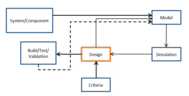
The foundations of engineering practice are mathematical models, the principles of physics, and empirical results obtained from experiments for defining design criteria. An engineer must know the laws of physics very well and use the relevant mathematical models and their solutions, either exact or numerical, to design parts, systems, and complex machines which function with certain reliability for an assumed lifetime. To help with this task, an engineer may use modelling tools to simulate the behavior of systems and their components. Modelling and the application of software tools are becoming increasingly common in modern engineering practice. As shown in Figure 1‑1, modeling and simulation results can help optimize and refine a design before the physical prototype is built. This minimizes the time required for the design process. In addition, application of modelling can minimize the final cost of a prototype or a product.
Modelling has a long history starting from ancient times when scientists used “equations” to relate variables or parameters to one another (e.g., Archimedes, Thales, Khawrazmi). Later, scientists and mathematicians developed “equations” which could represent the way that natural phenomena work and materials behave. These “equations” are sometimes referred to as laws of physics and constitutive equations since they are validated through time and the obtained results match with what we experience or measure in the real world with some approximations, of course. For example, Newton’s second law is given as a model which predicts the behaviour of material bodies under given forces applied to them, i.e., the relationship between forces applied to a body mass and the change of its momentum with respect to time.
Similarly, Ohm’s law is a model which relates the voltage across a resistor to the electrical current using the resistor’s material property. These models, and many other similar ones (e.g., Hooke’s, Fick’s, Fourier’s) related to different engineering disciplines, form the foundation of engineering. It is through their application that we trust the behavior and responses of our designs in the real world. Assume that we are flying in an airplane which is designed based on laws and governing equations or models applied to fluid mechanics and solid mechanics, among others. If we don’t trust and accept these laws and models, then it would not be logical to ride in an airplane!
Real-world phenomena are complex and usually involve many types of physics. For application in engineering, we usually simplify these phenomena and consider the dominant physics involved. For example, the length of a simple spring linearly changes under a given load according to Hooke’s law. But it becomes a more complex problem if the spring’s material behaves non-linearly, or if for example, electrical charges flow through it. Traditionally, the simplification of a problem is/was due to lack of tools for finding a solution which could represent more accurately that problem’s real world behaviour. It is at this point that modelling methods, e.g., Lagrangian and BG, and advanced modelling software tools, e.g., 20-sim, are valuable resources for finding solutions to complex engineering systems and optimizing our designs to have more economical, reliable, and durable products as end results. Although this book focuses on using bond graphs as a modelling method, we also emphasize the importance of learning and, hence, understanding the foundation and mathematics behind an energy-based approach for system analysis. For this purpose, we summarize Lagrangian mechanics in chapter 2 and provide some references for further reading.
The main body of the text is devoted to the BG method. This graphical (i.e., it can be sketched similar to engineering drawings) method translates the physical laws relevant to a desired system at hand into graphical interactions of interconnected assigned elements. The method uses laws of thermodynamics and the principle of cause and effect (in an acausal way) with the inclusion of constitutive relations relevant to system components.
In 1959, Henry M. Paynter at the MIT Department of Mechanical Engineering developed the bond graph method [1]. This method has fluctuated in application and popularity in the industry, with a recent rise due to its strength in modelling multi-energy-domain systems and the widespread availability of economically viable computer power [2].
In this book, we make use of facilities available in 20-sim, as a software tool for building, among others, BG models. 20-sim also offers solvers for finding solutions for the resulting system equations for simulation and design of systems. We use these solvers, with the modern script language SIDOPS++ included, to solve system equations as ordinary differential equations (ODEs). The system equations could be extracted from BG models or using Lagrangian method. The script language SIDOPS++ is suitable for complex system modelling and solving the relevant equations [3].
The reader may come across or already be familiar with other available methods/tools for modelling engineering systems, including block diagram, a signal processing graphical method; icon-diagram, a component-iconic graphical method; and advanced script languages/tools, e.g., Dymola, Smile, and recently Modelica [4], [5], [6].
2
In general, it is easier to perform engineering/technical calculations using a scalar quantity rather than a tensor/vector type quantity, mainly because a vector’s components depend on the selected coordinates system, and hence, more quantities to deal with. This was the main motivation for Joseph-Louis Lagrange (1736–1813), [7], [8] to start looking into the Newtonian mechanics close to a century after Newton developed his laws. Consequently, Lagrange developed a new formulation, so-called Lagrangian mechanics (1788).
Lagrange’s approach has advantages over that of Newton’s, specifically for analyzing complex multi-domain, multi-component systems. Lagrange’s approach releases us from having to consider a single inertia coordinates system and inter-component constraint forces. In addition, Langrangian method is faster and more efficient in terms of computation time and effort required to analyze and model engineering systems.
In Newtonian mechanics, a local condition, e.g., initial position and velocity (or momentum), is required for calculating the future states of a system. Using Newton’s law of motion, for a system or components of a system, the sum of forces (both applied,  and constrained/internal,
  ), is equal to the time rate of change of the momentum,
  .
.
(2.1) 
In order to identify the constraints, we usually isolate the components one by one from the rest of the system, while keeping the related dynamical equilibrium intact. This operation gives us the free-body diagram of each desired component, useful for analyzing the system’s motion dynamics and calculating inter-component constraint forces. However, in the Lagrangian approach, we consider a quantity that is like energy in dimension, the Lagrangian  , and use a set of partial differential equations (PDEs)—Euler-Lagrange or Lagrange’s equations— to analyze the system dynamics.
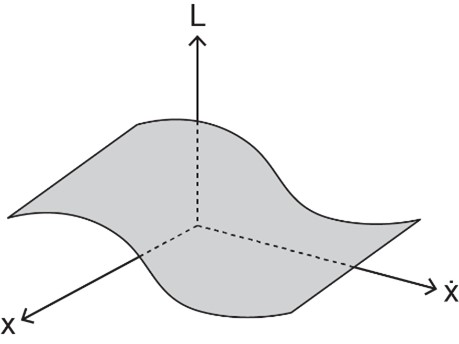
The latter is much more effective approach for analyzing the systems with many degrees of freedom and for dealing with multi-domain systems. In general, L is a function of coordinates considered and their time derivatives and, as well, could explicitly depend on time. For example, in a one-dimensional system, with designated coordinate x, the Lagrangian is written as  We can visualize as the topography of a surface represented by as a function of
  and
and  , as shown in Figure 2-1. This surface can vary with time, hence explicit dependence of on time, or it could be stationary. An example of the former is the motion of a mass particle on the surface of a moving sphere. Similarly, the Lagrangian of such a system is stationary if the sphere is not moving. The visualization presented in reference [9] may help readers with understanding Lagrangian surface.
 space
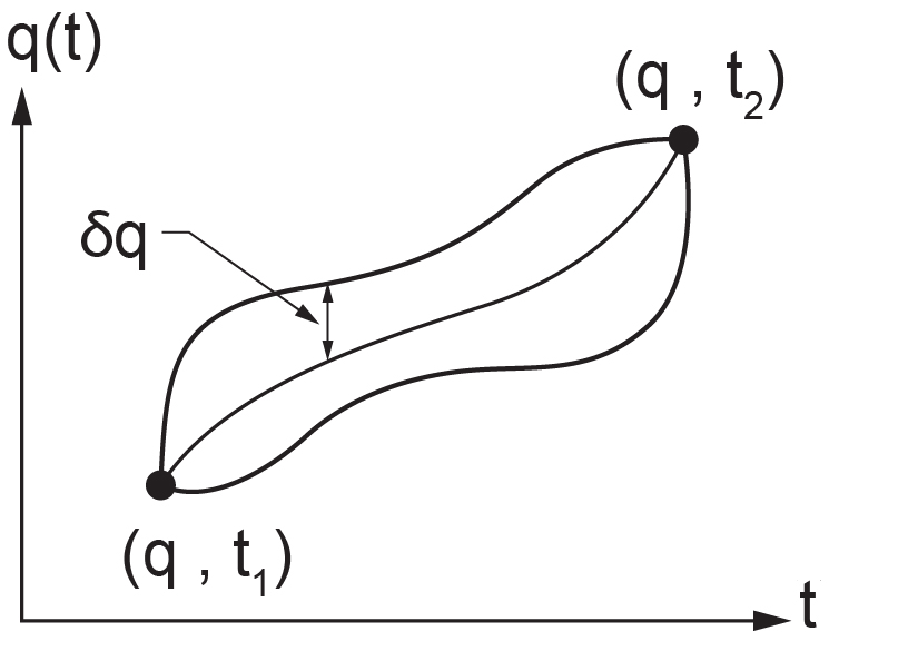
spaceThe foundation of Lagrangian mechanics rests on the principle of stationary action integral (also referred to as Hamilton’s principle) . This principle simply states that a system’s motion from a given state to another is such that a specific quantity (i.e., the system’s Lagrangian function) related to its motion is extremized (i.e., minimized or maximized); hence, the value of its integral (i.e., the action integral,  ) remains invariant [10].
 to
to  is such that the action integral has a stationary value for the actual path of the motion
In other words, among all possible paths available for the motion of the system to go through, there exists one specific path that minimizes/maximizes (for most systems minimizes; hence, this is also referred to a principle of least action) the integral of the corresponding Lagrangian with respect to time. Mathematically, the stationary action integral can be stated as
(2.2) ![\begin{equation*} \delta \mathcal{A} = \delta \left[ \int_{t_1}^{t_2} L(x,\dot x, t)dt \right] = 0 \end{equation*}](https://pressbooks.bccampus.ca/engineeringsystems/wp-content/ql-cache/quicklatex.com-344834e0991f50a49772686f4b0d25d2_l3.svg "Rendered by QuickLaTeX.com")
Using calculus of variations [11], [12], [13] and Equation (2.2) it can be shown (see section 2.5) that L should satisfy Lagrange’s equation, or
(2.3) 
where L is defined as  , with
  being the kinetic energy and
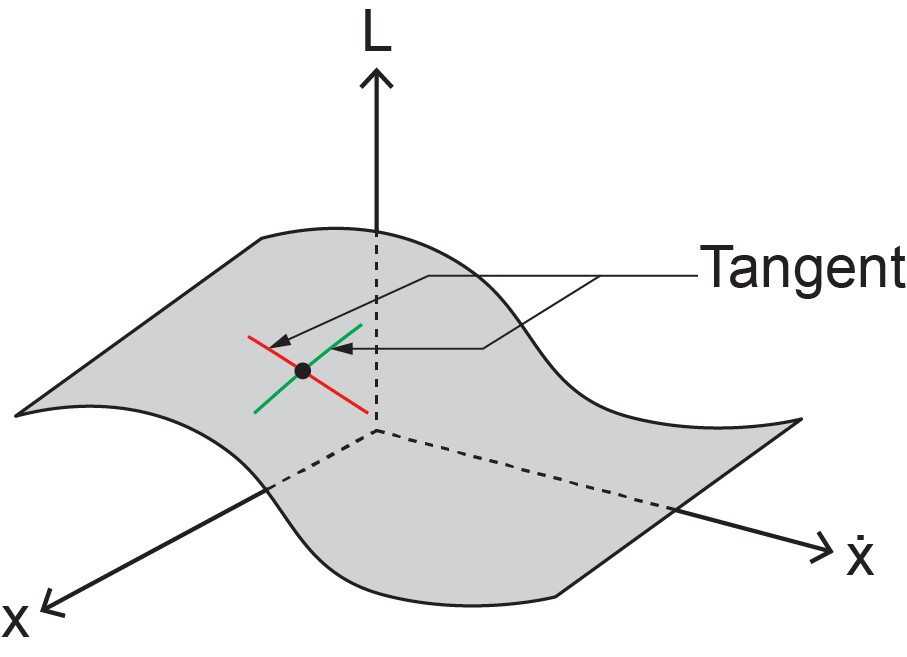
  the potential energy functions. With reference to Figure 2-1,
  is the slope at a selected point on the curve at the cross-section of surface and a plane parallel to -plane at desired , and
  is the rate of change in the slope at the same selected point on the curve at the cross-section of a plane parallel to -plane drawn from and including the selected point the same point. In other words, we draw two planes parallel to the and planes and equate their corresponding slopes at their intersectional point. Therefore, for a stationary point, these two quantities should be equal, as given by Euler’s equation (2.3). This is shown in the following sketch, see Figure 2-2.
By working out a simple example, we show that the Lagrangian approach is equivalent to the Newtonian approach in terms of the system’s equation of motion.
For this example, we show that Equation (2.3) gives the same results as that of Newton’s law of motion when applied to a simple mass-spring system, as sketched in Figure 2-3.
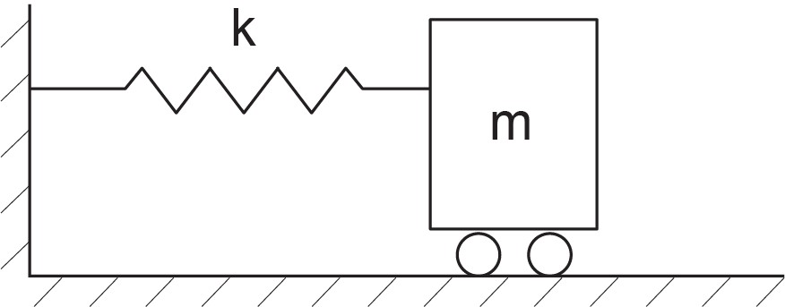
The kinetic energy for the mass  is
is  and the spring potential energy (i.e. stored elastic energy) with the spring constant k is
  . Therefore, using Equation (2.3), we get
 ![\dfrac{d}{dt} \left[ \dfrac{\partial}{\partial \dot x} \left(\dfrac{1}{2}m\dot x^2 - \dfrac{1}{2}kx^2 \right) \right] - \dfrac{\partial}{\partial x} \left(\dfrac{1}{2}m \dot x^2 - \dfrac{1}{2}kx^2 \right) = 0](https://pressbooks.bccampus.ca/engineeringsystems/wp-content/ql-cache/quicklatex.com-d95c10fd3e54c3ef6fd35149898e4bba_l3.svg "Rendered by QuickLaTeX.com") , or
, or  . Note that for this analysis we did not need to consider the free-body diagram of mass nor the spring force as the constraining force acting on it; rather, we used the scalar quantity
  . However, the assumption of having a potential function from which we can calculate the spring force is required (i.e.,
  ), see section 2.7.
In the following sections we expand on the Lagrangian method for discrete systems with related derivation, constraints and definitions for generalized coordinates, forces, and momenta.
We consider a particle with mass in a 3D space  , Cartesian system. By definition, the Lagrangian function is written as
  . We have assumed that the potential energy function is only a function of the space coordinates, so-called holonomic system. We now form two sets of derivatives
  and
and  of the Lagrangian function
  . Therefore, e.g., in 1D space, we have
  and
and  . Hence
  is a conservative force (see section 2.7). Now, using Newton’s second law, we can write the equation of motion, its -component, as
  or
or  and
and  Therefore,
  . Similar derivation can be performed for
  and
and  components of the equation of motion. Therefore, we get the Euler-Lagrange equations
(2.4) 
The motion of the particle could be considered, in principle, in another coordinate system, e.g., a cylindrical or spherical system, as well. Therefore, we can define a set of coordinates  to represent arbitrary coordinate systems, including Cartesian or curvilinear, and write Equation (2.4) in terms of
  , as well, for generality.
As mentioned previously, one of the advantages of Lagrangian method is that we do not require consideration of the constrained forces. Therefore, we can include only those coordinates that correspond to the degrees of freedom related to a system. This consideration leads us to the concept of generalized coordinates, which is used in Lagrangian mechanics instead of inertia coordinates used in the Newtonian mechanics.
We now define the generalized coordinates. First, we expand the system discussed in section 2.3 to include  number of particles that move in
  coordinate space, or
  . However, in a real-world system we can have restrictions imposed on the system’s motion; hence, some of the coordinates are constrained and do not vary independently. For example, a particle moving in a plane
  is constrained to move in -direction
  . Or, the mass bob of a pendulum moving in
  plane is restricted to move out of -plane and if the pendulum rod has a fixed length, then only coordinate
  varies during its motion. To capture these constraints, it is common and convenient to define generalized coordinates. Assume that for a coordinates system we have
  number of constraints. Therefore, the number of independent coordinates defining the motion is
  . By definition, for holonomic systems this is equal to the number of degrees of freedom [13]. Now we define the generalized coordinates as a subset of the original coordinates, with
  . Note that
  is the number of degrees of freedom which is equal to the number of generalized coordinates, and coordinates of the
  system are not necessarily the same as those of the , by one-to-one comparison.
For derivation of the equations of motion of a system, using Lagrangian approach, we can calculate  number of equations for the system, one by one, related to each generalized coordinate. We can also use the generalized coordinates to define the velocity-phase space, as the combined set of generalized coordinates and their corresponding time derivatives. Therefore, the Lagrangian, as a functional, reads
(2.5) 
Note that the time dependence of Lagrangian may be explicit for some systems and implicit for others and that the phase-space coordinates do not necessarily have the same units/dimensions. For example,  could be a displacement and
  an angle for a system like a pendulum with moving pivot point.
The fact that we can neglect the constrained coordinates in Lagrangian formulation is an advantage of this method over Newton’s because we don’t need to calculate the constrained “forces” in order to derive the equations of motion. Of course, the constrained forces can be calculated, if required, after having the solution to the system’s equations of motion.
Like the generalized coordinates, we also define associated generalized momenta and forces. As mentioned in the previous section, the definition of momentum in Lagrangian mechanics is more general than that of mass times the velocity. For example, it could be angular momentum, instead. Similarly, the definition of forces is not limited to mechanical forces; it can be applied, e.g., to voltage and temperature in electrical and thermal domains. Therefore, for each generalized coordinate we can define the corresponding generalized momentum and force. As given by Equation (2.6), we can write the generalized momenta and generalized force in terms of , as
(2.6) 
Section 2.7 discusses the topic of generalized force in terms of its types: conservative and non-conservative.
Hamilton’s principle, as given by Equation (2.2), is basically a mathematical expression of calculus of variations application for a system dynamical motion with the realization that Lagrangian functional is the function that should be extremized [12]. Therefore, Lagrange’s equations are resulted from the related calculations, naturally. This realization was first expressed by William Rowan Hamilton (1805-1865), [14], [11], [15].
Equation (2.4) can be written in terms of generalized coordinates, as
(2.7) 
Equation (2.7) shows that Lagrange’s equation is consequence of, and necessary for, making the action integral stationary. We assume that variation  results from variation in one of the arbitrarily selected coordinates,
  (dropping the subscript index for simplicity without losing the generality) while satisfying the fixed boundary conditions, or
  . Obviously, the same operation can be performed for all coordinates involved,
  .
.
 for an arbitrary
 Substituting Equation (2.7) into Equation (2.2), after dropping the subscript index and assuming  for simplicity, we get
![\begin{equation*} \delta \mathcal{A} = \delta \Big\{ \int_{t_1}^{t_2} \left[ \frac{d}{dt} \left( \frac{\partial L}{\partial \dot q} \right) - \frac{\partial L}{\partial q} \right] dt\Big\} = \Bigg\{ \int_{t_1}^{t_2} \delta \big\[\underbrace{\left[ \frac{d}{dt} \left( \frac{\partial L}{\partial \dot q} \right) - \frac{\partial L}{\partial q} \right]}_{L} \big\ dt \Bigg\} = 0 \end{equation*}](https://pressbooks.bccampus.ca/engineeringsystems/wp-content/ql-cache/quicklatex.com-46a4c7858d29f053da7696e5171c7e60_l3.svg "Rendered by QuickLaTeX.com")
But  and the last term can be written as
  and hence,
 ![\delta L = \left[ \dfrac{\partial L}{\partial q} - \dfrac{d}{dt} \left(\dfrac{\partial L}{\partial \dot q} \right) \right] \delta q + \dfrac{d}{dt} \left( \dfrac{\partial L}{\partial \dot q} \delta q \right)](https://pressbooks.bccampus.ca/engineeringsystems/wp-content/ql-cache/quicklatex.com-2711aa9630f548aa98c44955112ff9b2_l3.svg "Rendered by QuickLaTeX.com") .
.
Back substituting into action integral expression, we get ![\delta \mathcal{A} = \int_{t_1}^{t_2} \left[ \dfrac{\partial L}{\partial q} - \dfrac{d}{dt} \left( \dfrac{\partial L}{\partial \dot q} \right) \right] \delta q \: dt + \int_{t_1}^{t_2} \dfrac{d}{dt} \left( \dfrac{\partial L}{\partial \dot q} \delta q \right) dt = 0](https://pressbooks.bccampus.ca/engineeringsystems/wp-content/ql-cache/quicklatex.com-dbec2b1c54535b2f414ce9ab10b71a82_l3.svg "Rendered by QuickLaTeX.com") .
.
But the last integral gives ![\int_{t_1}^{t_2} \dfrac{d}{dt} \left( \dfrac{\partial L}{\partial \dot q} \delta q \right) dt = \dfrac{\partial L}{\partial \dot q} \delta q \Big|_{t_1}^{t_2} = \dfrac{\partial L}{\partial \dot q} \bigg[ \underbrace{\delta q (t_2) - \delta q(t_1)}_{=0} \bigg] = 0](https://pressbooks.bccampus.ca/engineeringsystems/wp-content/ql-cache/quicklatex.com-15273469054b07de4ccf371eee47e001_l3.svg "Rendered by QuickLaTeX.com") .
.
Therefore, we have ![\delta \mathcal{A} = \int_{t_1}^{t_2} \left[ \dfrac{\partial L}{\partial q} - \dfrac{d}{dt} \left( \dfrac{\partial L}{\partial \dot q} \right) \right] \delta q \: dt = 0](https://pressbooks.bccampus.ca/engineeringsystems/wp-content/ql-cache/quicklatex.com-3b0fc29a446a63dacc6223f5758cf0a2_l3.svg "Rendered by QuickLaTeX.com") . Since is arbitrarily selected, the integrand should be equal to zero in order to have the value of the integral null, or
. Since is arbitrarily selected, the integrand should be equal to zero in order to have the value of the integral null, or  . This concludes the derivation of Lagrange’s equation using Hamilton’s principle. However, one can derive Lagrange’s equation in a more direct way using calculus of variations or virtual work principles, see [11], [13], [16].
So far, we have considered systems that do not involve energy dissipation. In practice, however, we require extra terms in Lagrange’s equation to account for friction existing in real-world systems. Therefore, we expand the discussion to include non-conservative forces, e.g., friction and dampers, and find the corresponding Lagrange equation, including related topics such as cyclic coordinates, symmetry, multi-domain, and higher-order systems, [8], [13], [17].
From Equation (2.6), it can be shown that if Lagrangian function does not have explicit dependency on one of the coordinates, say  , among all , then the conjugate momentum
  is conserved. The proof is as follows. Writing the Lagrange’s equation for coordinate , we have
  . Since by definition, is not a function of , then
  . Therefore,
  , and written in terms of generalized momentum , we get
  , or is invariant with respect to time, hence conserved. It is common to call the coordinate , cyclic or ignorable.
The generalized forces can be conservative or non-conservative. Conservative forces are those like gravity, buoyancy, mechanical spring, electrostatic, and magnetic. Non-conservative forces are those like friction, damping, and resistance.
By definition, a conservative force is curl free, or  . Writing this expression in index notation, we have
  , where
  is the permutation symbol [18]. For example, force under gravity is
  . Calculating the curl gives
  . Each term is identically zero; hence, the force under gravity field is conservative. Now, using the vector identity
  or
or  ; i.e., the curl of a gradient of a scalar function is identically zero, and we can write a conservative force as the gradient of a scalar, such as potential function V as
  . By convention, the negative sign indicates that potential energy increases when work is done against a force field and vice versa.
We now, write Equation (2.7), after dropping the index  for simplicity, for
  and
and  . Therefore,
  , or
, or  But
But  , and we get
  . This is the equation of motion (i.e.
  ). We clearly see that the conservative force is already included in the Lagrange equation given by Equation (2.7). Now, for the case that we have a non-conservative force, or that the potential function is a function of velocity
  and q, (i.e.
  or
or  ), then we can write use Equation (2.7) to write
  Re-arranging the term in this expression, we get
  We define the expression on the right-hand side as the non-conservative force, as
  Hence,
  Again, we have shown that the non-conservative force is already included in the Lagrange equation given by Equation (2.7), provided a modified potential function is defined, as given by
  . See reference listed at [11] for more details.
In section 2.7, we discussed the applicability of Lagrange’s equation given by Equation (2.7) for conservative and non-conservative forces. In practice, we could benefit from a more explicit form of the Lagrange equation whose terms can be easily identified for different types of forces, including energy dissipation such as damping and resistance. In this way, we can readily calculate the related terms in the Lagrange equation for modeling and simulation of a desired system.
There are several possible ways to derive the Lagrange equation using, e.g., principles of virtual work and d’Alembert’s principle, directly from Newton’s second law of motion and first law of thermodynamics or energy conservation (e.g., conservation of sum of kinetic and potential energies) [8], [11], [13], [15], [17].
We use the conservation of energy approach to derive the alternative form of Equation (2.7) including its expansion [17].
We consider the kinetic energy of a system with generalized coordinates for  ) (see section 2.4) represented by
  and its potential energy by
  . Note that, as we discussed previously, for many mechanical systems kinetic energy is a function of
  and potential energy a function of , only. Therefore, the resulted Lagrange equation can be simplified, accordingly. Now, using conservation of total energy of the system, we can write
(2.8) 
But  and
and  , using their functional relationships. After substituting into Equation (2.8), we get
  . Note that the Einstein summation convention applies, or
  . Now, using the relation for the kinetic energy of the system, or
(2.9) 
where  is defined as the generalized mass matrix, a diagonally nonzero matrix, corresponding to the generalized coordinates. Therefore, its diagonal elements could be mass or moment of inertia when the generalized coordinates are displacement and angle, respectively. For example, for a
  system, we have:
 .
.
After expanding the expression in the bracket on the R.H.S., we get:
 .
.
With having  and
and  , and
, and  , particle mass,
  , inertia, and
  we get
  Now, differentiating T with respect to , we get
  and substituting into Equation (2.9), we get
  Now, we calculate total change of T using the last expression, or
  But we had,
  Therefore, subtracting these last two relations, gives, after simplification,
  But we can manipulate the first term on the right-hand side as
  Substituting into the last relation for dT, we get
(2.10) ![\begin{equation*} dT = \left[ \frac{d}{dt} \left( \frac{\partial T}{\partial \dot q_i} \right) - \frac{\partial T}{\partial q_i} \right] dq_i \end{equation*}](https://pressbooks.bccampus.ca/engineeringsystems/wp-content/ql-cache/quicklatex.com-780770b01eecae93d54669e6badf8e19_l3.svg "Rendered by QuickLaTeX.com")
Now, substituting Equation (2.10) into (2.8), we get ![\left[ \dfrac{d}{dt} \left( \dfrac{\partial T}{\partial \dot q_i} \right) - \dfrac{\partial T}{\partial q_i} \right] dq_i + dV = 0.](https://pressbooks.bccampus.ca/engineeringsystems/wp-content/ql-cache/quicklatex.com-96505c4a5668e82fd8014b1297749b71_l3.svg "Rendered by QuickLaTeX.com") Now, if
Now, if  i.e. holonomic systems, then we get
  and, after substitution, we have
 ![\left[ \dfrac{d}{dt} \left( \dfrac{\partial T}{\partial \dot q_i} \right) - \dfrac{\partial T}{\partial q_i} + \dfrac{\partial V}{\partial q_i} \right]dq_i = 0.](https://pressbooks.bccampus.ca/engineeringsystems/wp-content/ql-cache/quicklatex.com-804ea904ae17d092a98a7d506ee4f4df_l3.svg "Rendered by QuickLaTeX.com") This expression is true for any arbitrarily selected
This expression is true for any arbitrarily selected  ; therefore, the terms in the bracket should be identically null, or
(2.11) 
Equation (2.11), is an alternative form of Lagrange’s equation and holds when forces associated with the system are conservative, included in the  term. Note that using Lagrangian, and Equation (2.11) we can recover Equation (2.7). The inclusion of non-conservative generalized forces,
  (usually the loading associated with each coordinate) should be added to the right-hand side of Equation (2.11). Also, energy dissipation due to viscous damping or resistance is usually given as
  and contributes to Lagrange equation as
  . Finally, we get the alternative form of Lagrange equation, as
(2.12) 
Recall the n is the number of generalized coordinates. In matrix form, Equation (2.12) can be written as

Lagrangian method can be applied to many kinds of engineering systems, including mechanical, electrical, thermal, hydraulic, and their possible combinations as multi-domain systems. As discussed in the previous sections, the established concept of generalized coordinates, momenta, and force are key tools to model such systems.
System equations are mostly second-order differential equations, like Newton’s second law, and Kirchohff’s law for RCL circuits. Previous sections, e.g., Equation (2.7), presented Lagrange’s equation for such systems. One may require, mostly in continuous systems, to build the Lagrangian function for higher-order systems, e.g., fourth-order bi-harmonic equation for fluid flows or plate displacements. Fortunately, the Lagrangian method can be easily extended to cover the higher-order systems by considering a Lagrangian function, as given by Equation (2.13)
(2.13) 
Using the calculus of variations and Hamilton’s principle, we can derive the corresponding Lagrange’s equation [13], [9]. This s done by:
(2.14) 
where m is the differentiation order; e.g., for  , we have

Worked-out examples are useful to demonstrate applications of Lagrangian method. These examples, for mechanical and electrical systems, appear below. Each example includes numerical values assigned to the parameters and presents simulation results. Selected examples include accompanying screen-recorded video files demonstrating the solution steps for related system equations using 20-sim. After learning from the related video file, the reader can modify the parameters and run the simulation for specific design cases.
We want to find the equations governing its motion dynamics for the system sketched in Figure 2-5. For this example, we neglect the effect of gravity.
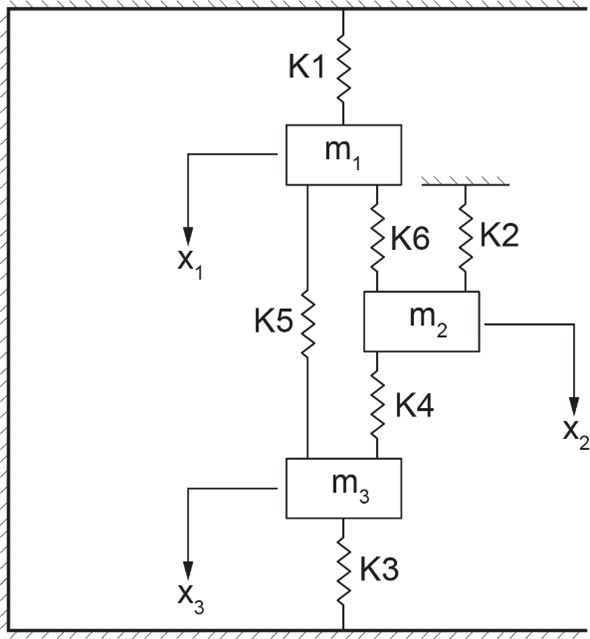
This system has three degrees of freedom  associated with three masses
  . For three masses,
  , and each can move vertically; hence, the number of constraints is
  for each mass. This gives
  . The Lagrangian method is used to find the equations of motion, or three coupled second-order differential equations. We start by writing the kinetic and potential energy expressions of the system and forming the corresponding Lagrangian. The kinetic energy of the system is
  ). For the potential energy, we should use the difference in displacements associated with each spring because the neutral position of the unstressed springs do not contribute to the potential energy. For example, for the spring
  , connecting masses
  and
and  , we should use
  as the variable, or
  . Therefore, the potential energy of the system consisting of the sum of all springs is
  . Note that for this system the kinetic energy is a function of only
  and potential energy a function of
  . Applying Euler-Lagrange equation to each mass, or degree of freedom, we get a system of ODEs, written in matrix form,

For example, the Euler-Lagrange equation associated with mass reads  . But we have
  and
and  . Having information about initial and boundary conditions for displacements and/or velocities, we can obtain the solution of the system’s equations using 20-sim. An initial velocity of 0.2
  is applied to mass
  , for example. The script code is as follows:
parameters
real m1 = 15.0 {kg};
real m2 = 30.0 {kg};
real m3 = 15.0 {kg};
real k1 = 50.0 {N/m};
real k2 = 100.0 {N/m};
real k3 = 50.0 {N/m};
real k4 = 20.0 {N/m};
real k5 = 70.0 {N/m};
real k6 = 10.0 {N/m};
variables
real x1 {m};
real x2 {m};
real x3 {m};
real x1_dot {m/s}; // velocity
real x2_dot {m/s}; // velocity
real x3_dot {m/s}; // velocity
real x1_dot_dot {m/s2}; //acceleration
real x2_dot_dot {m/s2}; //acceleration
real x3_dot_dot {m/s2}; //acceleration
real Fk1 {N}; // force spring k1
real Fk2 {N}; // force spring k2
real Fk3 {N}; // force spring k3
equations
x1_dot_dot = -(1/m1)*((k1+k5+k6)*x1-k6*x2-k5*x3);
x2_dot_dot = -(1/m2)*((k2+k4+k6)*x2-k6*x1-k4*x3);
x3_dot_dot = -(1/m3)*((k3+k4+k5)*x3-k4*x2-k5*x1);
x1_dot = int (x1_dot_dot , 0);
x2_dot = int (x2_dot_dot , 0.2); //initial velocity 0.2m/s
x3_dot = int (x3_dot_dot , 0);
x1 = int (x1_dot , 0.2); //initial displacement 0.2m
x2 = int (x2_dot , 0);
x3 = int (x3_dot , -0.1); //initial displacement -0.1m
Fk1 = k1*x1;
Fk2 = k2*x2;
Fk3 = k3*x3;
The results for displacements of the masses and velocities are shown below, see Figure 2-6.
Here is a video showing how to build and run the model for this example in 20-sim:
We consider a system with two degrees of freedom, as shown in Figure 2-7. The damping coefficients  and
and  and spring stiffness
  and
and  are used to calculate the potential and damping functions and
  , respectively.
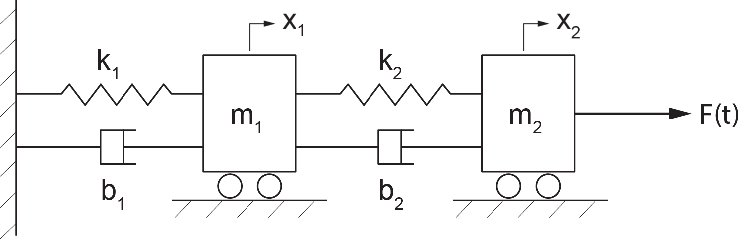
The non-conservative Rayleigh energy dissipation function is,  . The derivative of this function with respect to
  gives the damping forces associated with mass
  . The kinetic energy is
  , and potential energy reads
Lagrange’s equation for motion of mass reads  and for mass is
  . Performing the derivatives, we get
Using Lagrange’s equation, with , we get the equations of motion of the system in matrix form as

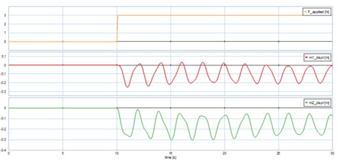
We use 20-sim to solve the systems equations. A step function is used for applied force. The script code is as follows:
parameters
real m1 = 2.0 {kg};
real m2 = 1.0 {kg};
real k1 = 20.0 {N/m};
real k2 = 30.0 {N/m};
real b1 = 0.1 {N.s/m};
real b2 = 0.05 {N.s/m};
real start_time = 10 {s};
real amplitude = 0.5;
variables
real x1 {m};
real x2 {m};
real x1_dot {m/s};
real x2_dot {m/s};
real x1_dot_dot {m/s2};
real x2_dot_dot {m/s2};
real F_applied {N}; // applied force
equations
x1_dot_dot = -(b1+b2)/m1*x1_dot+b2/m1*x2_dot-(k1+k2)/m1*x1+k2/m1*x2;
x2_dot_dot = -(1/m2)*(-b2*x1_dot+b2*x2_dot-k1*x1+k2*x2+F_applied);
x1_dot = int (x1_dot_dot , 0);
x2_dot = int (x2_dot_dot , 0);
x1 = int (x1_dot , 0);
x2 = int (x2_dot , 0);
F_applied = amplitude*step (start_time);
The results for displacements of the masses and applied force are shown below, see Figure 2-8.
Here is a video showing how to build and run the model for this example in 20-sim:
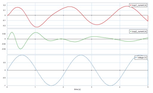
For this example, we consider an electrical circuit with two loops/branches. For the system, we have; electric charges and ; resistors  and
and  ; inductors
  ,
,  , and
, and  ; and capacitors
  and
and  as Figure 2-9 shows. The voltage source is
  , connected to loop 1.
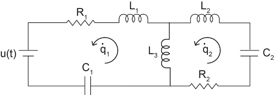
For comparison with a typical mechanical system, the equivalent of mass is an inductor; for spring, a capacitor; and for damper, a resistor. Therefore, using the Lagrangian method, we can write the kinetic energy of the system as  . Note that electric charge is analogous to mechanical displacement and electric current to velocity, or
  and
and  . Therefore, e.g., the term
  represents the stored kinetic energy in the corresponding inductor. Similarly, the potential energy is
  . Note that the capacitance is the inverse of stiffness, or
  . The energy dissipation function for the system is
  . Using Langrange’s equation,
  , gives the electric circuit system equations as

One can use rate of charge or the electric current, I as the variable by replacing  in the system’s equations. This gives
  and
and  where
where  and
and  are the voltage across the capacitors, respectively.
We use 20-sim to solve the system equations. The script code is as follow
parameters
real L1 = 0.15 {H};
real L2 = 0.2 {H};
real L3 = 0.25 {H};
real C1 = 0.05 {F};
real C2 = 0.02 {F};
real R1 = 1 {ohm};
real R2 = 2 {ohm};
real omega = 3 {rad/s};
real amplitude = 1;
variables
real q1 {C};
real q2 {C};
real q1_dot {A};
real q2_dot {A};
real q1_dot_dot ;
real q2_dot_dot ;
real Voltage {V}; // applied voltage
equations // equations are manipulated
q2_dot_dot*(L1*L2+L2*L3+L1*L3)=-L3*R1*q1_dot-(L1+L3)*R2*q2_dot-L3/C1*q1-(L1+L3)/C2*q2+Voltage*L3;
q1_dot_dot*(L3) = (L2+L3)*q2_dot_dot+R2*q2_dot+(1/C2)*q2;
q1_dot = int (q1_dot_dot , 0);
q2_dot = int (q2_dot_dot , 0);
q1 = int (q1_dot , 0);
q2 = int (q2_dot , 0);
Voltage = amplitude*sin (omega*time);
Typical plots for current in each loop is shown in Figure 2-10 for a sinusoidal voltage.
Atwood’s machine is a collection of pulleys and masses. This example examines and models the dynamical behavior of this machine as shown in Figure 2-11.
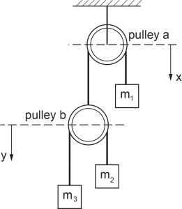
This system has two degrees of freedom  describing the motion of mass and pulley b. Therefore, two ODEs describe the system dynamical behaviour. The massless un-stretchable string length hanging over pulley
  is
is  , and that of pulley
  is
is  . We measure the potential energy with reference to the top of pulley with vertical displacement designated with and similarly from top of pulley with , as shown in Figure 2-11. The kinetic energy reads
  , where , using the geometrical constraints and string lengths,
  . Therefore,
  . Substituting in kinetic energy relation, gives
 ![T= \dfrac{1}{2} [m_1 \dot x^2 + m_2 (\dot y - \dot x)^2 + m_3 (\dot y + \dot x)^2 ]](https://pressbooks.bccampus.ca/engineeringsystems/wp-content/ql-cache/quicklatex.com-216a57e4ace1327fadedc034a824a2a4_l3.svg "Rendered by QuickLaTeX.com") . The potential energy reads
. The potential energy reads  . After substituting for
  , and
, and  and algebraic simplifications we get
  , where constant C is given by
  . The Langrange equations in terms of and are
  and
and
 , having
![\begin{equation*} L = T - V = \dfrac{1}{2} [m_1 \dot x^2 + m_2 ( \dot y - \dot x)^2 + m_3 (\dot y + \dot x)^2 ] -xg(m_2 + m_3 - m_1) - yg(m_3 - m_2) \end{equation*}](https://pressbooks.bccampus.ca/engineeringsystems/wp-content/ql-cache/quicklatex.com-449471c56fa7d517d84766ad62960799_l3.svg "Rendered by QuickLaTeX.com")
We dropped  , since its differentiation is zero. Hence,


Substituting into the corresponding Lagrange equations, we get the system’s equations of motion as

To simplify the equations, eliminate  by multiplying the first equation by
  and the second one by
  . After some manipulations, we get

We use 20-sim to solve these system equations. The script code is as follows:
parameters
real m1 = 1.0 {kg};
real m2 = 2.0 {kg};
real m3 = 4.0 {kg};
real g = 9.81 {m/s2};
variables
real x {m};
real y {m};
real x_dot {m/s};
real y_dot {m/s};
real x_dot_dot {m/s2};
real y_dot_dot {m/s2};
equations
/* x_dot_dot = (1/(m1+m2+m3))*(-y_dot_dot*(m3-m2)+g*(m1-m2-m3)); */
x_dot_dot = g*(m1-m2-m3)*(m2-m3)/(m1*m2+m1*m3+4*m2*m3);
y_dot_dot = (1/(m3+m2))*((x_dot_dot+g)*(m2-m3));
x_dot = int (x_dot_dot , 0);
y_dot = int (y_dot_dot , 0);
x = int (x_dot , 0);
y = int (y_dot , 0.1);
In the analysis of Atwood’s machine, the pulley and string are usually considered massless. In this example, we include these parts, assuming the string having mass  , total length
  , and linear mass density
  and the pulley with mass
  , radius
  , and moment of inertia
  [19].
[19].
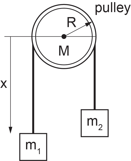
2Datum for potential energy is a horizontal plane at the level of the pulley’s centre. From the datum, the length of hanging string on the two sides of pulley is  . The potential energy is due to the masses and the string mass, or
  . Note that x is measured downward from the datum toward mass . The kinetic energy is due to the masses, string, and the pulley’s angular kinetic energy,
  with angular velocity
  . Therefore,
  . The Lagrangian is written as

The Lagrange is equation reads , or  , after substituting
  . The result reduces to the familiar result of
  for massless string and pulley
  .
.
We use 20-sim to solve these system equations. The script code is as follows:
parameters
real Ms = 2.5 {kg}; // string mass
real L = 2.0 {m}; //string length
real M = 3.0 {kg}; //mass of the pulley
real R = 30.0 {cm}; //radius of the pulley
real g = 9.81 {m/s2}; // grav. acceleration
real m1 = 4.0 {kg};
real m2 = 1.5 {kg};
variables
real x {m}; //vertical displacement
real I {kg.m2}; // pulley moment of inertia
real x_dot {m/s}; // vertical velocity
real x_dot_dot {m/s2}; // vertical acceleration
equations
I = 0.5*M*R^2;
x_dot_dot = g*(m1-m2+(Ms/L)*(x-L))/((m1+m2+(Ms/L)*(L+ pi*R)+I/R^2));
x_dot = int (x_dot_dot , 0.0);
x = int (x_dot , 0);
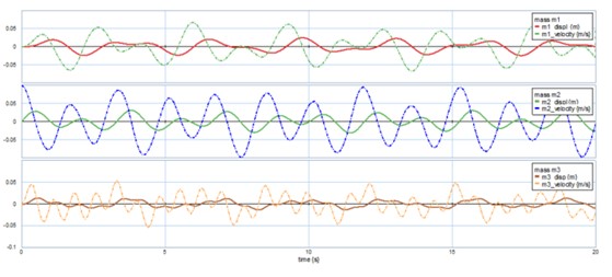
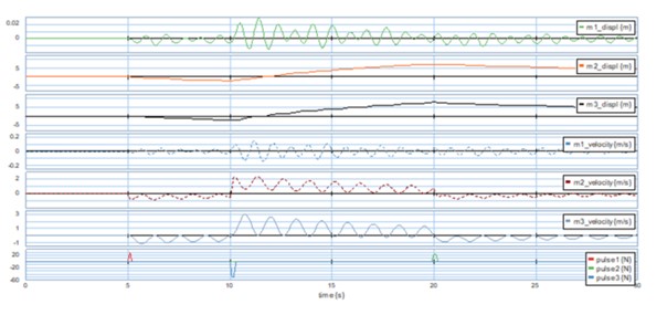
For this example, we consider a mechanical system with three degrees of freedom,  , associated with three masses,
 . The arrangement of springs and dampers is shown, with their coefficients, in Figure 2-13, with corresponding stiffness
  and damping
  coefficients. An applied force,
  acting on mass and all wall contact surfaces are considered to have negligible friction.
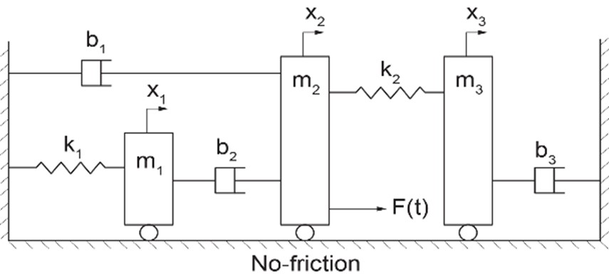
The kinetic energy of the systems reads  and the potential energy is
  . Similarly, the damping function reads
  . The Lagrange’s equations are
  , with
because the applied force is exerted on mass . Performing the differentiations, we can write the equations of the system, as

and  . In matrix form, the system’s equations are

We use 20-sim to solve these system equations. The applied force is composed of three impulses applied at 5, 10, and 20 second. The script code is as follows:
parameters
real m1 = 1.0 {kg};
real m2 = 3.0 {kg};
real m3 = 2.0 {kg};
real k1 = 50.0 {N/m};
real k2 = 30.0 {N/m};
real b1 = 0.1 {N.s/m};
real b2 = 0.2 {N.s/m};
real b3 = 0.3 {N.s/m};
variables
real x1 {m};
real x2 {m};
real x3 {m};
real x1_dot {m/s};
real x2_dot {m/s};
real x3_dot {m/s};
real x1_dot_dot {m/s2};
real x2_dot_dot {m/s2};
real x3_dot_dot {m/s2};
real F_applied1 {N};
real F_applied2 {N};
real F_applied3 {N};
equations
x1_dot_dot = -b2/m1*x1_dot+b2/m1*x2_dot-k1/m1*x1;
x2_dot_dot = -(1/m2)*(-b2*x1_dot+(b1+b2)*x2_dot+k2*x2-k2*x3+F_applied1+F_applied2+F_applied3);
x3_dot_dot = -(1/m3)*(b3*x3_dot-k2*x2+k2*x3);
x1_dot = int (x1_dot_dot , 0);
x2_dot = int (x2_dot_dot , 0);
x3_dot = int (x3_dot_dot , 0);
x1 = int (x1_dot , 0);
x2 = int (x2_dot , 0);
x3 = int (x3_dot , 0);
F_applied1 = 3*impulse (5,0.1);
F_applied2 = 5*impulse (20,0.2);
F_applied3 = -10*impulse (10,0.2);
Sample results are shown in Figure 2-14.
Here is a video showing how to build and run the model for this example in 20-sim:
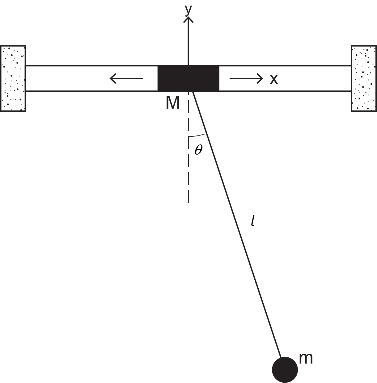
A simple pendulum with mass hanging from a free-moving pivot with mass . The system has two degrees of freedom: oscillation of pivot,  and pendulum motion about vertical designated by angle
  . The pendulum string with length is massless and unstretchable. We consider the datum at the pivot level and gravitational acceleration
  pointing downwards, as in Figure 2-15.
Mass coordinates read  ; hence, the velocity components are
  . We can write kinetic energy of the system as
![\begin{equation*} T = \frac{m}{2} \left[ (\dot x + l \dot \theta \text{cos} \theta)^2 + (l \dot \theta \text{sin} \theta )^2 \right] + \frac{M}{2} \dot x^2 = \frac{m}{2} (\dot x^2 + l^2 \dot \theta ^2 + 2l \dot x \dot \theta \text{cos} \theta) + \frac{M}{2} \dot x^2 \end{equation*}](https://pressbooks.bccampus.ca/engineeringsystems/wp-content/ql-cache/quicklatex.com-053b4889ad915ab79ccebe63018db523_l3.svg "Rendered by QuickLaTeX.com")
Similarly, the potential energy of the systems reads  . Note that the pivot motion is horizontal with coordinates (x, 0). The Lagrange equation for rotational motion with respect to coordinate reads
  , or
, or  . After simplification, we get
  . Note that for fixed pivot (or
  ) we get the familiar result for a simple pendulum. The Lagrange equation for translational motion with respect to coordinate reads
  , or
, or  . After performing differentiation, we get
  . Collectively, the system’s equations of motion are

We use 20-sim to solve these system equations. An initial velocity of 0.5 rad/s is applied to the pendulum. The script code is as follows:
parameters
real m = 0.5 {kg}; // pendulum/bob mass
real M = 1.0 {kg}; // pivot mass
real g = 9.81 {m/s2}; //gravity
real L = 30 {cm}; //pendulum length
variables
real x {m};
real x_dot {m/s};
real x_dot_dot {m/s2};
real theta {rad};
real theta_dot {rad/s};
real theta_dot_dot {rad/s2};
equations
x_dot_dot = (1/cos (theta))*((g/L)*sin (theta)-theta_dot_dot);
theta_dot_dot = (1/(m*L*cos (theta)^2-M-m))*(m*L*sin (theta)*cos (theta)*theta_dot^2-g/L*(m+M)*sin (theta));
x_dot = int (x_dot_dot , 0);
x = int (x_dot , 0);
theta_dot = int (theta_dot_dot , 0.5);
theta = int (theta_dot , 0);
Sample results are shown in Figure 2-16.
Here is a video showing how to build and run the model for this example in 20-sim:
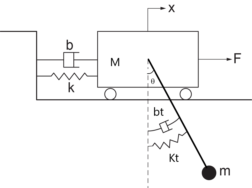
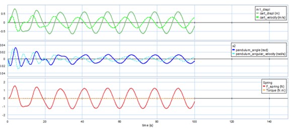
In this example we consider a system consisting of a pendulum with its pivot attached to the centre of a freely moving mass . The mass is connected to a spring with stiffness  and a damper with damping coefficient . The pendulum bob has a mass of and is attached to a torsional damper with damping coefficient
  and a torsional spring with stiffness
  . The pendulum string is massless and has a length of . We consider the datum at the pivot level and gravitational acceleration pointing downwards, as in Figure 2-17. The system has two degrees of freedom; oscillation of pivot,
  and pendulum motion about vertical direction designated by angle .
The coordinates of mass read  , and its velocity components are
  . We can write kinetic energy of the system as
![\begin{equation*} T = \frac{m}{2} \left[ (\dot x + l \dot \theta \text{cos} \theta )^2 + (l \dot \theta \text{sin} \theta )^2 \right] + \frac{M}{2} \dot x^2 = \frac{m}{2} (\dot x^2 + l^2 \dot \theta ^2 + 2l \dot x \dot \theta \text{cos} \theta ) + \frac{M}{2} \dot x^2 \end{equation*}](https://pressbooks.bccampus.ca/engineeringsystems/wp-content/ql-cache/quicklatex.com-c237beb14cfebcfef8505ccf7129207a_l3.svg "Rendered by QuickLaTeX.com")
Similarly, the potential energy of the system reads  . The damping function of the system is
  .
.
The Lagrange equation for rotational motion with respect to coordinate reads  , or
, or  . After simplification, we get
  . The Lagrange equation for translational motion with respect to coordinate reads
  , or
, or  . After performing differentiation, we get
  . Collectively, the system’s equations of motion are

We use 20-sim to solve these system equations. The script code is as follows:
parameters
real m = 0.5 {kg}; // pendulum/bob mass
real M = 1.0 {kg}; // pivot mass
real g = 9.81 {m/s2}; //gravity
real L = 30 {cm}; //pendulum length
real k = 2 {N/m}; // spring stiffness
real kt = 0.5 {N.m/rad}; // torsional stiffness
real bt = 0.5 {N.m.s/rad}; // torsional damping
real b = 0.2 {N.s/m}; // damping
real amplitude = 1; // amplitude of applied force
real omega = 0.5 {rad/s}; // frequency of applied force
variables
real x {m};
real x_dot {m/s};
real x_dot_dot {m/s2};
real theta {rad};
real theta_dot {rad/s};
real theta_dot_dot {rad/s2};
real F_applied {N};
real F_spring {N}; // linear spring force
real T_spring {N.m}; // torsional spring torque
real y; // aux. variable, to help the solver
equations
x = int (x_dot , 0);
x_dot = int (x_dot_dot , 0);
theta = int (theta_dot , 0);
theta_dot = int (theta_dot_dot , 0);
y = -m*L*cos (theta)*(theta_dot_dot);
x_dot_dot = (1/(m+M))*(m*L*sin (theta)*theta_dot^2 + y -k*x-b*x_dot+F_applied);
theta_dot_dot = -g/L*sin (theta) -1/L*cos (theta)*x_dot_dot -1/(m*L^2)*(bt*theta_dot+kt*theta);
F_applied = amplitude*sin (omega*time);
F_spring = k*x;
T_spring = kt*theta;
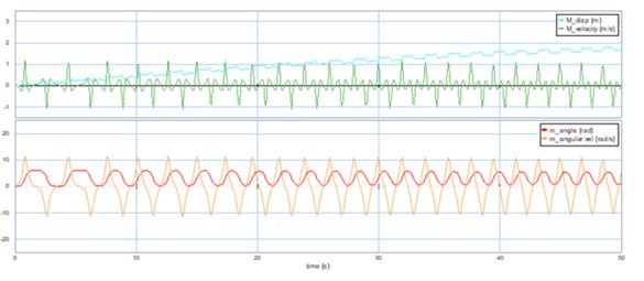
Cart displacement, pendulum angle, and force and torque of the springs are shown in Figure 2-18.
Here is a video showing how to build and run the model for this example in 20-sim:
Figure 2-19 shows a particle with mass sliding on a circular ring with radius . The ring itself is rotating about the -axis with a constant angular velocity  . We want to find the equation of motion for the mass particle.
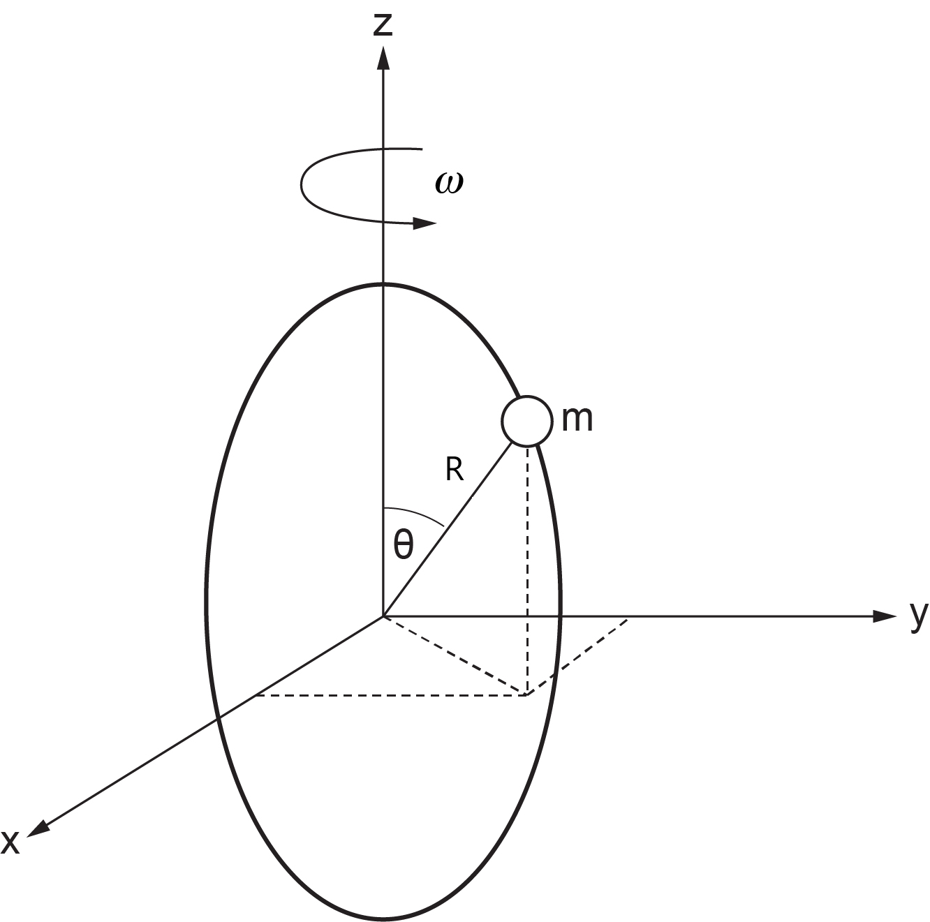
The generalized coordinate is , the polar angle. We can write the coordinates of the mass particle as  ,
,  , and
, and  . Therefore,
  ,
,  , and
, and  . Therefore, the kinetic energy reads
  ) and after substitution of velocities and simplifications we get
  . Similarly, the potential energy of the mass particle reads
  . Note that the kinetic energy of the particle consists of those resulted from angular velocity
  , defined in spherical coordinates in the
  plane due to sliding of the mass on the circular ring, and the rotational velocity
  , defined in a
  plane parallel to the
  plane at any given time during the motion.
Now we can write the Lagrange’s equations, using Equation (2.12), with the assumption that no friction and non-conservative forces exist, or  . Hence
  . But
. But  ,
,  and
and  . After substitution and rearranging the terms, we get the equation of motion for the mass particle as

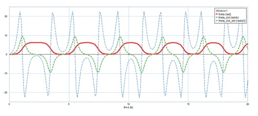
We use 20-sim to solve these system equations. An initial angular velocity of 0.2 rad/s is applied to the mass. The script code is as follows:
parameters
real g = 9.81 {m/s2}; //grav. acc.
real R = 40 {cm}; //ring radius
real omega = 0.8 {rad/s}; // ring angular velocity
variables
real theta {rad};
real theta_dot {rad/s};
real theta_dot_dot {rad/s2};
equations
theta_dot_dot= ((1/2)*omega^2*sin (2*theta)+g*sin (theta)/R);
theta_dot = int (theta_dot_dot , 0.0);
theta = int (theta_dot , 0.2);
The angular displacement, velocity and acceleration are shown in Figure 2-20.
Here is a video showing how to build and run the model for this example in 20-sim:
Figure 2-21 shows a load with mass is carried by a robotic arm in the plane. The length  of the arm and its angle with respect to -axis are functions of time
  , or
, or  and . The damping coefficients for radial and tangential motions are
  and , respectively.
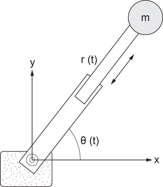
The generalized coordinates (or degrees of freedom) are  , and corresponding velocities are
  , for mass . We can write the kinetic energy as
  , due to radial and tangential velocities, respectively. The potential energy, with reference to the support, is
  . The damping function is
  . The conservative gravity force due to the load mass is accounted for through the potential function . The force
  and torque
  exerted by the robot-arm motor to move the mass are components of generalized force vector, or
  . Now, we have
  ,
,  ,
,  ,
,  ,
,  ,
,  ,
,  and
and  . Using Equation (2.12), we can write the equations of the motion for the mass , as

We use 20-sim to solve the system equations. The script code is as follows:
parameters
real m = 0.5 {kg}; // load mass
real g = 9.81 {m/s2}; //grav. acc.
real bt = 0.5 {N.m.s/rad}; // tangential damping
real br = 0.2 {N.s/m}; // radial damping
variables
real arm {m};
real arm_dot {m/s};
real arm_dot_dot {m/s2};
real theta {rad};
real theta_dot {rad/s};
real theta_dot_dot {rad/s2};
real F {N}; //applied force
real T {N.m}; // applied torque
equations
arm_dot_dot = (arm*theta_dot^2-g*sin (theta)-br*arm_dot/m+F/m);
theta_dot_dot = (1/(m*arm^2))*(-2*m*arm*arm_dot*theta_dot-m*g*arm*cos (theta)-bt*theta_dot+T);
arm_dot = int (arm_dot_dot , 0);
arm = int (arm_dot , 0.2);
theta_dot = int (theta_dot_dot , 0);
theta = int (theta_dot , 0);
F = sin (0.2*time);
T = 0.2;
Exercises
 and
and  ) of mass and for an initial condition of at
  . Also draw the phase diagram (i.e.,
  vs. ) for each mass. Assume that the strings are massless and inextensible.
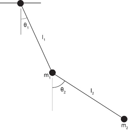
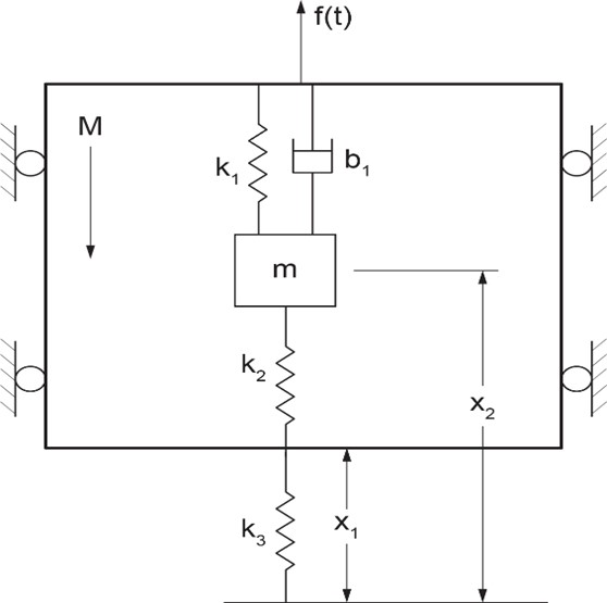
and is supported by a spring  and moving vertically, guided by frictionless rollers under load . The subsystem is composed of a mass m, two springs and , and a damper , as shown in the figure below. The gravitational acceleration vector is directed downward,
  .
. 
 . Modify the model provided for this example accordingly and run the simulation.
 between mass and the wall. Modify the model provided for this example accordingly and run the simulation.
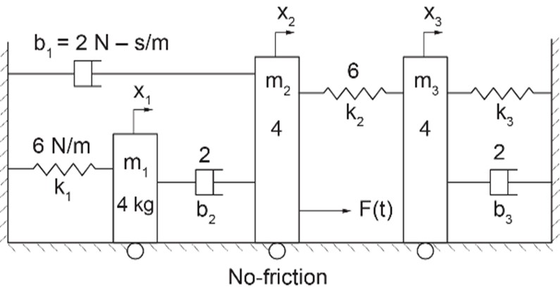

3
All engineering systems share the physical phenomenon of the transfer and distribution of energy among their corresponding components while converting one form of energy to another. The balance of energy “flowing” through a system should be maintained. The total amount of energy remains constant—energy is conserved—according to the first law of thermodynamics. In 1959, Henry Paynter used the first law and common system features to create a general graphical method for analyzing and modelling multi-domain engineering systems. His objectives were mainly to have a unified graphical method for modelling single- and multi-domain systems as well as a common procedural algorithm to develop such models and obtain their relevant systems’ equations. Hence, the bond graph (BG) method was created [1], [20], [21], [22].
BG represents a system through graphical modelling. The BG method assigns ports (the communication point) for each component of a system and connects each port to the adjacent component through bonds (the communication path and direction) for a two-way energy/power exchange. At any instant of time, each component either receives (sends) a quantity called effort and simultaneously sends (receives) another quantity called flow. The product of the quantities of effort and flow has the dimension of power—or time rate of energy change. In a mechanical system, force is the effort and velocity is the flow; in an electrical system, voltage is the effort and current is the flow. The collection of bonds—with the inclusion of the related system components’ constitutive laws, constraints, and boundary conditions—forms the system BG model. Building a BG model requires nine basic elements, defined as follows. See section 3.4 for full description.
The nine basic BG elements, along with the principle of causality, can be employed for building a BG model representing a given system’s dynamical behaviour (see further sections for detailed explanation). The resulting BG model, then, would clearly show the kinematic (i.e., continuous stream of flow) and kinetic (i.e., continuous stream of effort) of the system and can be used to extract the equations governing the dynamical behaviour of the whole system. In addition, the insights provided by a BG model are valuable for understanding the physics/dynamics of the system and provide a powerful tool for simulation, design, and optimization of the system. The procedure for building a BG model is similar for analogous engineering systems. For example, when the parameters of the pertinent components are used, the BG model for a mechanical mass-spring-damper system is identical to those of an electrical resistor-capacitor-inductor (RCL) system.
In this chapter, we discuss, among other topics, the definitions for basic BG elements, the causality principle and assignments, and the concept of state variables.
The components of a system can be categorized according to energy transfer through the system into three types. These are kinetic energy storages, potential energy storages, and energy dissipaters. In addition, we have energy source/sink components acting with the surroundings at the boundary of the system. There may also exist components that simply transfer energy without storing or dissipating it. Finally, a system may include components, such as a distributor, that perform as junctions. Figure 3‑1 shows a sketch of a mechanical system with examples of component categories, as mentioned above. All these types of components can be modelled using nine basic BG elements, as discussed in further sections.
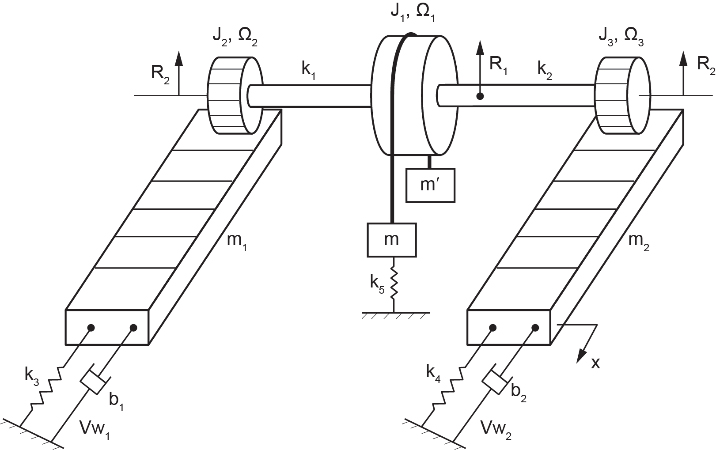
The dynamical behaviour of a system changes with time. Therefore, time rate of energy or power is the quantity of interest in BG models. The relation between energy  and power
  can mathematically be written as
(3.1) 
We can identify the components of a given system as “lumped” entities that exchange energy with one another. Using the first law of thermodynamics, we can write the change in energy as the sum of work  and heat
  exchanges, or
  . Summing up the energy changes of lumped components in a system gives the total energy change of the system. For example, without losing generality, we consider a mechanical system component receiving power and exhibiting a displacement
  and velocity
  . Using Equation (3.1), the amount of energy in terms of work input can be written as
  . But the work is also equal to the force times the displacement; hence,
  . Substituting for
  , we get
  . Considering and as the time limits associated with the duration of energy transfer, we can, after integrating, write the work as
(3.2) 
where is mass. In a BG model, each system component is designated by a suitable basic element and associated port(s). Depending on the type of element used, the number of ports could be one, two, or more. The power direction is designated by a half-arrow ( ) which shows the direction of power to or from the port for each element. Traditionally, half-arrows are used in BG models to keep the full-arrow shape for one-way signal data, as in block diagram graphs.
As mentioned above and by Equation (3.2), for mechanical systems, the power is composed of two quantities: force and velocity. In BG method, we generalize this concept and show the power with the product of  and , the effort and flow, respectively. Hence, the product of effort and flow has the dimension of power, or
  . For example, for a rotational motion, is the torque and is the angular velocity (see Table 3‑1). In other words, in a BG model, the kinetics of a system is modelled by transfer of the efforts of its components according to the equilibrium, and the kinematics by transfer of components’ flows according to compatibility requirement. We will discuss this feature of BG method, using some examples, in section 4.6.
Figure 3‑2 shows the definition of power direction for element A sending power to B, and the associated effort, shown above the half-arrow, and flow, shown, by definition, below the half-arrow.
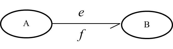
| Systems | Effort () | Flow () | Displacement | Momentum |
| mechanical-translational | force [N] | velocity [m/s] | distance [m] | [kg.m/s] |
|---|---|---|---|---|
| rotational mechanical | torque [N.m] | angular velocity [rad/s] | angle [rad] | angular momentum [kg.m2/s] |
| hydraulic | pressure [Pa] | volume flow rate [m3/s] | volume [m3] | hydraulic momentum [Pa.s] |
| thermal/thermodynamics | temperature [K] | entropy change rate [J/ K.s] | entropy [J/K] | — |
| thermo-fluid | enthalpy (specific) [J] | mass flow rate [kg/s] | mass flow [kg] | flow momentum |
| electrical | voltage [V] | current [A] | charge [C] | flux linkage [V.s] |
| magnetics | magnetic force [A] | magnetic flux rate [Wb/s] | magnetic flux [Wb] | — |
| chemical | chemical potential [J/mol] | mole flow rate [mol/s] | mole flow [mol] | — |
To establish the principle of cause and effect relationship in BG method, we use the definition of causality assignment. The cause signal brings all the history data to the system/element, and through the dynamical behaviour of the system, the present signal effect is decided and provided as output.
As mentioned, in BG method, the half-arrow indicates the direction of power between related elements in a BG model. However, the half-arrow does not provide information about the direction of power constituents, i.e., effort or of the flow. In principle, we can arbitrarily define these directions. For example, in Figure 3‑2, we can assign direction pointing from component A to B (hence, should be directing from B to A) or vice versa. In other words, the causality assignment is a symmetrical one. By definition, a small transverse/vertical line, a causality stroke, is drawn close to one of the ports at the power bond to show the direction of effort toward it, hence the direction of flow away from it, as shown in Figure 3‑3. This operation is critical for building BG models and, in terms of providing a definite solution, has consequences in the resulting equations of the system. After the causality is assigned, then the signal received by the element is the cause, and the returning signal—or the element response—is the effect.
The preferred causality assignment is called integral causality, and the alternative option is the derivative/differentiate causality. We will discuss the details further in section 3.5.
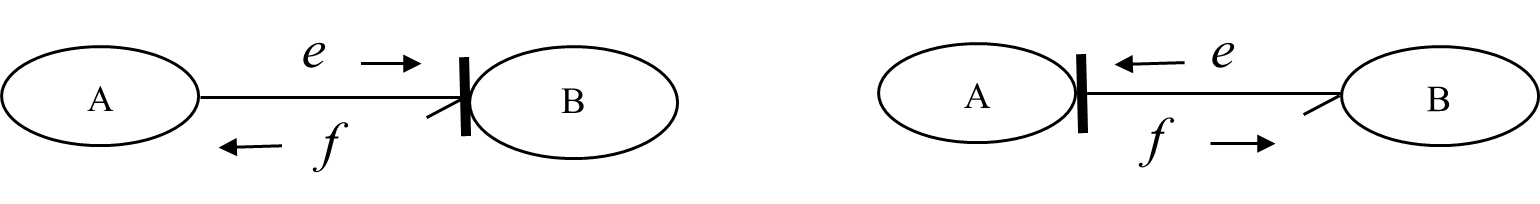
As mentioned in the previous section, building a BG model of a physical system involves consideration of the energy conservation, transfer, and conversion through the system. In a BG model, we focus on the rate of energy or power as the quantity to deal with.
For energy storage, we define two elements, represented by (inertial element) for kinetic energy and (capacity element) for potential energy storages. For energy dissipation, we define one element, represented by (friction or resistor element). We represent the energy source/sink acting at the boundary of the system by two elements, one for effort  and one for flow
  . To manage the distribution of energy through the system, we define two elements as junctions, represented by junction 1 and junction 0. For energy transfer/conversion, we define two elements, represented by transformer
  and gyrator
  . Therefore, in total, we have nine elements available and sufficient for building a BG for any given physical system, with the inclusion of their modulated versions (
 ,
,  , etc.) for when a signal is input to the corresponding element from an external source. Examples of physical/engineering systems are mechanical, electrical, thermal, hydraulic systems, or some hybrid systems composed of subsystems assembled of different energy media.
Each one of the BG elements mentioned above should behave according to the relevant physical laws represented by their constitutive relations—a mathematical model. For example, a linear mechanical spring is modelled by element , whose governing equation should comply with Hooke’s law. However, a given spring can go under deformation either by receiving an effort (i.e., force) or a flow (i.e., displacement rate/velocity). Depending on the system and computational preferences, we can assign causality strokes to the element to specify that the desired spring receives effort or flow. This rule, the causality assignment, must be applied to all bonds in a BG model. Examples of typical translational mechanical elements are shown in Table 3‑2.
| -element (damper) | -element (spring) | -element (mass) | -element (lever) | -element (gyroscope) |
 | 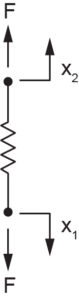 | 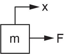 | 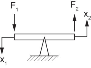 | 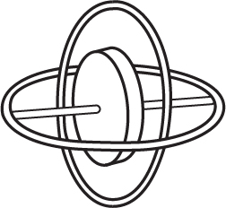 |
In the next sections, we will define the constitutive equations, preferred causality, and physical representation examples for all nine BG elements.
In BG modelling, the -element is a passive element; it should receive power to return a signal. This requirement means that the half-arrow power bond should be drawn toward this element. An -element has only one port for communicating to the rest of the system. Examples are mass bodies in mechanical systems and inductors in electrical systems.
As shown in Figure 3‑4, the input quantity for the -element can be either effort () or flow (); consequently, the response is flow or effort, respectively. Note that the causality stroke (the vertical/transverse line) specifies the direction of effort defined to be toward the stroke; hence, the direction of flow is to be away from it. We use red colour for specifying non-integral causality strokes.
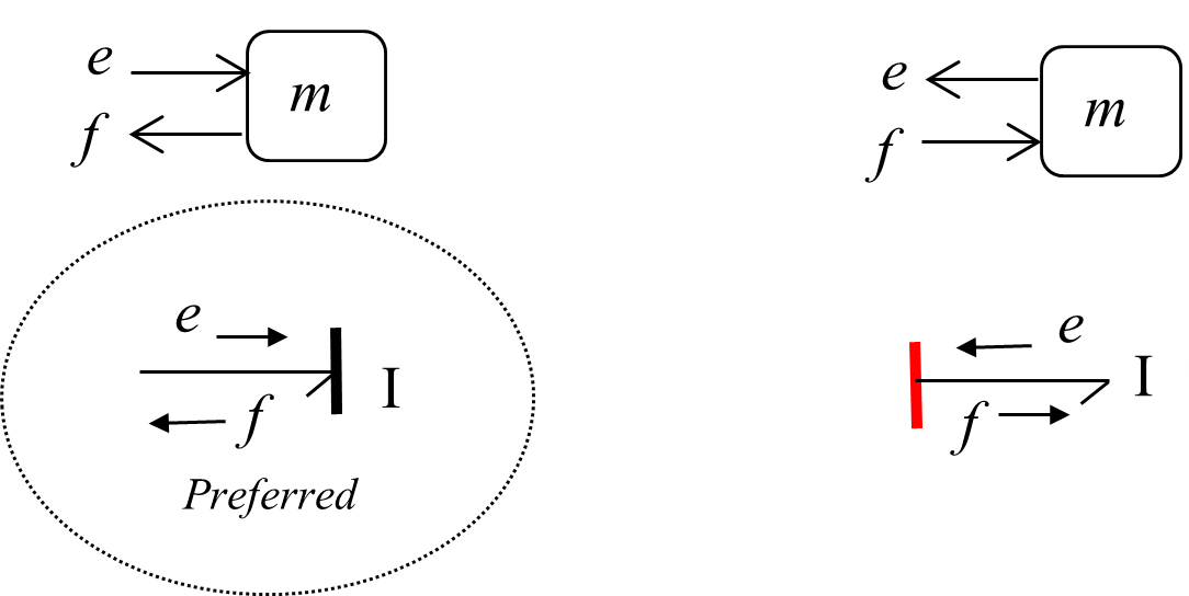 -element, with preferred integral causality indicated by dashed circle (left) and derivative causality (right)
Now the question is, how do we choose between these two possible options when building a BG model? What are the implications when choosing one option versus the other? The short answer is that both options are legitimate, but there is a preference for having the -element receiving the effort and sending the flow out—integral causality—hence, the causality stroke is placed at the half-arrow head at the port close to the element. The effort is the cause, and the flow is the effect relevant to -element when it is integrally causalled.
-element, the preferred causality assignment is effort-in, so-called integral causality.Mathematically, the statement given in the box can be analyzed as follows. In a mechanical system, for example, we consider a point mass and apply Newton’s second law to the motion of that point mass. Therefore, we can write  (
( is net applied force, and
  is the velocity of the mass), or in BG generalized notation,
  . Recall that the symbol represents effort (force) and represents flow (velocity) in a mechanical system (see Table 3‑1). We also use the symbol , representing mass , or inductance for electrical systems. Now, for the effort-in option that we have, since the input should be ,
  or after integration,
  Note that the integral of force with respect to time is the momentum
  , (
, ( ). The equation
  is the key point here. Let’s see what it means. The flow (velocity) is equal to momentum divided by the mass. This is well-known! In BG method, however, it has an important meaning: for the -element, the input effort quantity, after being integrated, is divided by the -element parameter , and the output quantity is flow or velocity. This can be shown in a block/signal diagram along with equivalent BG model diagram (see Figure 3‑5). Since the integration of effort is involved, we call the related causality assignment an integral causality which is preferred for -elements. From the physical point of view, the integration of effort collects all the input data and hence represents a more comprehensive description of the system in terms of modelling. In addition, the resulting system’s equations (see section 3.5) are first-order ODEs when integral causality is assigned.
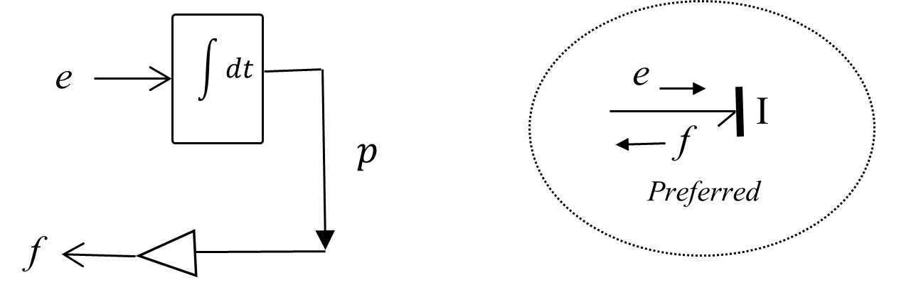 -element with assigned integral causality and state variable
 The constitutive equation for the -element in a BG model is given as
(3.3) 
The momentum , which is the result of input/effort integration, is a state variable (see section 3.5).
Now, we consider the second possible option with flow-in signal (see Figure 3‑4). We have  . This equation matches with the input and output data, since the time derivative of input flow, given on the right-hand side of the relation, multiplied by the -element parameter is the element output or effort, given on the left-hand side. This is the derivative causality assignment since the derivative of input data is involved. This case can be shown in a block diagram along with equivalent BG model diagram (see Figure 3‑6).
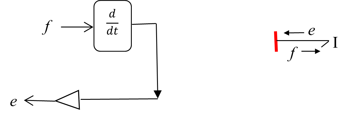 -element with assigned derivative causality
In BG modelling method, the -element is a passive element because it should receive power to react to. This requirement means that the half-arrow power bond should be drawn toward this element. A -element has only one port for communicating to the rest of the system. Examples are springs in mechanical and capacitors in electrical systems. As shown in Figure 3‑7, the input quantity can be either effort () or flow (); consequently, the response is flow or effort, respectively. Note that the causality stroke (the vertical line) specifies the direction of effort defined to be toward the stroke; hence, the direction of flow is to be away from it.
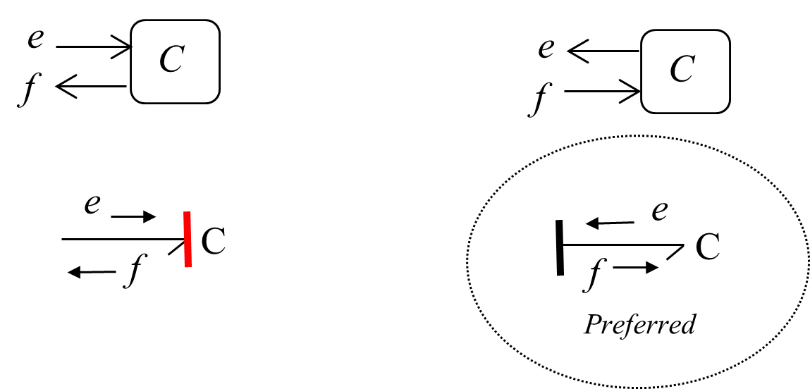 -element, with preferred one indicated by dashed circle, integral causality (right) and derivative causality (left)
Now the question is, how do we choose between these two possible options when building a model? What are the implications when choosing one option versus the other? The short answer is that both options are legitimate, but there is a preference for having the -element sending the effort and receiving the flow—integral causality—hence, the causality stroke is placed at the opposite end of the half-arrow head away from the element’s port.
-element the preferred causality assignment is effort-out, so-called integral causality.Mathematically, the statement given in the box can be analyzed as follows. In a mechanical system, e.g., we consider a linear mechanical spring with stiffness and apply Hooke’s law to its motion. Therefore, we can write  ( is net applied force, and is the displacement) or, in generalized BG notation,
  , where
  the spring compliance. Recall that the symbol represents effort (force) and represents flow (velocity) in, e.g., a mechanical system, (see Table 3‑1). We use the symbol
  , representing spring compliance or capacitance in electrical systems as well.
Now, for the effort-out option having the flow as the input, we can write  . That is, for the -element, the input flow quantity, after integration, is divided by the -element’s compliance and gives the output quantity as effort . For -element, the displacement
  , which is the result of input/flow integration, is the state variable.
(3.4) 
This can be shown in a block/signal diagram along with equivalent BG model diagram (see Figure 3‑8).
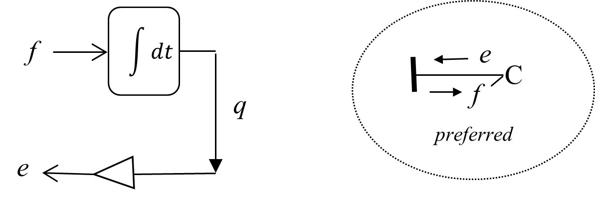 -element with assigned integral causality and state variable
 Now, we consider the second possible option with effort-in signal (see Figure 3‑7). We can write  , with effort being the input and displacement as the output data; hence, the time derivative of output displacement () is required to get the flow/velocity. This is derivative causality assignment, since the derivative/differential operation is needed to get the output signal involved. This case can be shown in a block diagram along with equivalent BG model diagram (see Figure 3‑9).
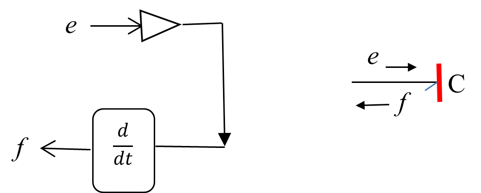 -element with assigned derivative causality
In BG modelling method, the -element is a passive element since it should receive power to return a signal. This requirement means that the half-arrow power bond should be drawn toward this element. An -element has only one port for communicating to the rest of the system. Examples are dampers in mechanical and resistors in electrical systems.
As Figure 3‑10 shows, the input quantity for the -element can be either effort () or flow (); consequently, the response is flow or effort, respectively. Note that the causality stroke (the vertical line) specifies the direction of effort defined to be toward the stroke; hence, the direction of flow is to be away from it.
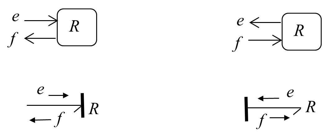 -element
There is no preference for having the -element receiving the effort or the flow. Therefore, the causality stroke can be placed at either end of the half-arrow power connection, according to the causality requirement for the adjacent elements.
-element, there is no preferred causality assignment- i.e., it is neutrally causalled.Mathematically, the statement given in the box can be analyzed as follows. In a mechanical system, for example, we consider a damper with viscous damping coefficient . The constitutive equation gives the force applied on the damper proportional to the rate of displacement. Hence, we can write  ( is net applied force, and is the velocity). Writing in BG generalized notation,
  . Now, for the effort-in option we have, since the input should be ,
Now, we consider the option with flow-in data (see Figure 3‑10). We have . Since the constitutive equation for a linear viscous damper is algebraic, we do not need to integrate or differentiate the input signal to obtain the output signal for an -element. Therefore, there is no preference, and -element is neutrally causalled. Figure 3‑11 shows block diagrams along with equivalent BG model diagram with causality assignments for an -element.
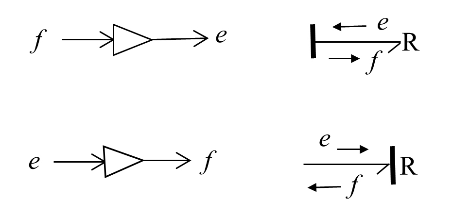 -element with assigned causality
In BG modelling method, the boundary source elements are of two types. The sources for effort (such as force, voltage) and flow (such as velocity, current) are represented by and respectively. These elements are active, and the half-arrow power bond should be drawn from these sources to the connecting elements in the system. Source elements have only one port each, for communicating to the rest of the system. As shown in Figure 3‑12, the causality assignments are uniquely assigned for these elements.
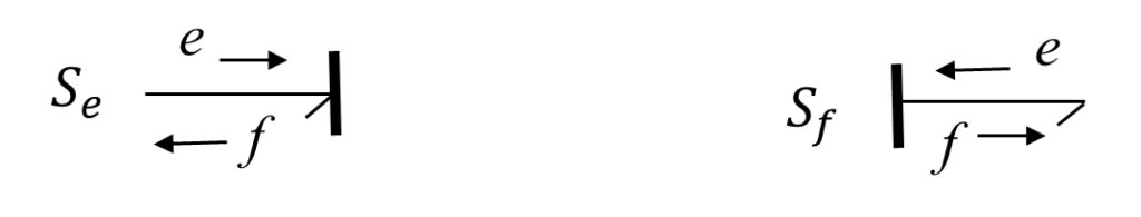
In BG modelling method, system-required constraints for distribution of energy are applied using two elements. These are multi-port elements with symbols “1” and “0” that can receive or send power to the elements connecting to them. This requirement means that the half-arrow power bond can be drawn toward or from these elements.
A 1-junction is a flow equalizer or an effort summator element. For example, in a mechanical system, a common node with connecting system components exhibits the same value of velocity, or the elements of an electrical circuit experience the same value of current. The causality assignment for a 1-junction element must comply with its definition of distributing the flow received through one of the connecting bonds to the rest of bonds. Therefore, only one bond can send flow to a 1-junction—the strong bond—and the remaining connecting bonds should send the same flow to connecting elements; hence, the causalities are assigned accordingly, as shown in Figure 3‑13.
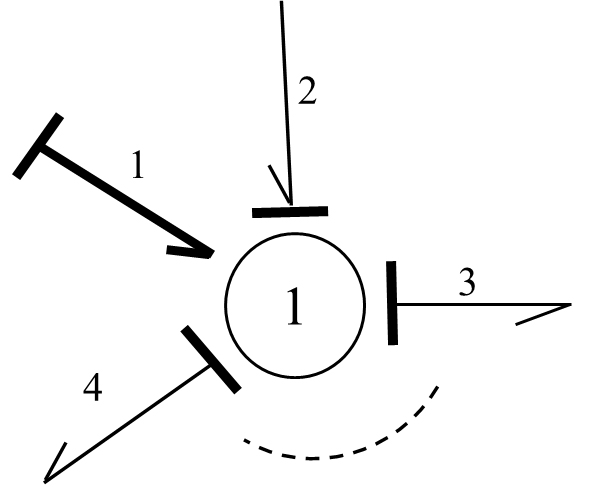
After labelling the bonds with arbitrary numbers, we can write the conservation energy law, in terms of its rate, as  . But the 1-junction distributes the flow received from the strong bond (i.e., the bond labelled “1”) equally to bonds 2, 3, and 4. Hence,
  . From these relations, after substitution, we get
  . Similarly, for number of bonds connecting to a 1-junction, we have the constraint relations for the 1-junction as
(3.5) 
In Equation (3.5), the summation for efforts received by 1-junction is algebraic, or the input power is considered to be positive, and the output power has a negative sign.
A 0-junction is an effort equalizer or a flow summator element. For example, in a mechanical system, a common node with connecting system components experiences relative velocity values or the nodes in an electrical circuit with common voltage. The causality assignment for a 0-junction element must comply with its definition of distributing the effort received through one of the connecting bonds to the rest of bonds. Therefore, only one bond can send effort to a 0-junction—the strong bond—and the remaining connecting bonds should send the same effort to connecting elements, hence, the causalities are assigned accordingly, as shown in Figure 3‑14.
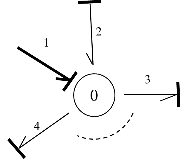
After labelling the bonds with arbitrary numbers, we can write the conservation energy law, in terms of power or energy rate, as  . But the 0-junction distributes the effort received from the strong bond (i.e., the bond labelled “1”) equally to bonds 2, 3, and 4. Hence,
  . From these relations, after substitution, we get
  . Similarly, for number of bonds connecting to a 0-junction, we have the constraint relations for the 0-junction as
(3.6) 
In Equation (3.6), the summation for flows received by the 0-junction is algebraic, or the input power is considered to be positive and the output power has a negative sign.
In physical engineering systems, energy may be converted by some components while its conservation is maintained. Examples are levers and gearbox in mechanical systems or electrical transformers and motors in electrical systems. In BG modelling method, there exist two elements for modelling convertors: transformer and gyrator . These elements are two-port elements and can receive power through one of their ports as input and deliver a converted power from the other port as output, in terms of the power variables effort and flow. The causality assignments determine the directions of flows and efforts as being inputs or outputs. In this section, we present the details of -element followed by those of -element.
A transformer element, represents the converter that receives the same type of physical quantity as the type it delivers, after conversion. For example, a force applied at one end of a lever is converted to a magnified/reduced force at the other end, or the velocity of the lever’s end point is converted to another velocity value related to another point proportional to their distances from the lever’s pivot.
As shown in Figure 3‑15, a -element can have one effort and one flow as inputs, and consequently, delivers converted corresponding effort and flow as outputs. The conversion parameter  should be defined, based on the physical system data. For example, for the case that flow
  is the input and flow
  the output, we can write
  to define . But from energy conservation we have
  , or the output effort
  . Similarly, for the case that effort
  is the input and effort
  the output, we can write
  , using . But from energy conservation, we have, or the output flow
  .
.
These relations constitute the -element equations and are shown in Figure 3‑15, for each case where the inputs to the -element are identified with thick arrows.
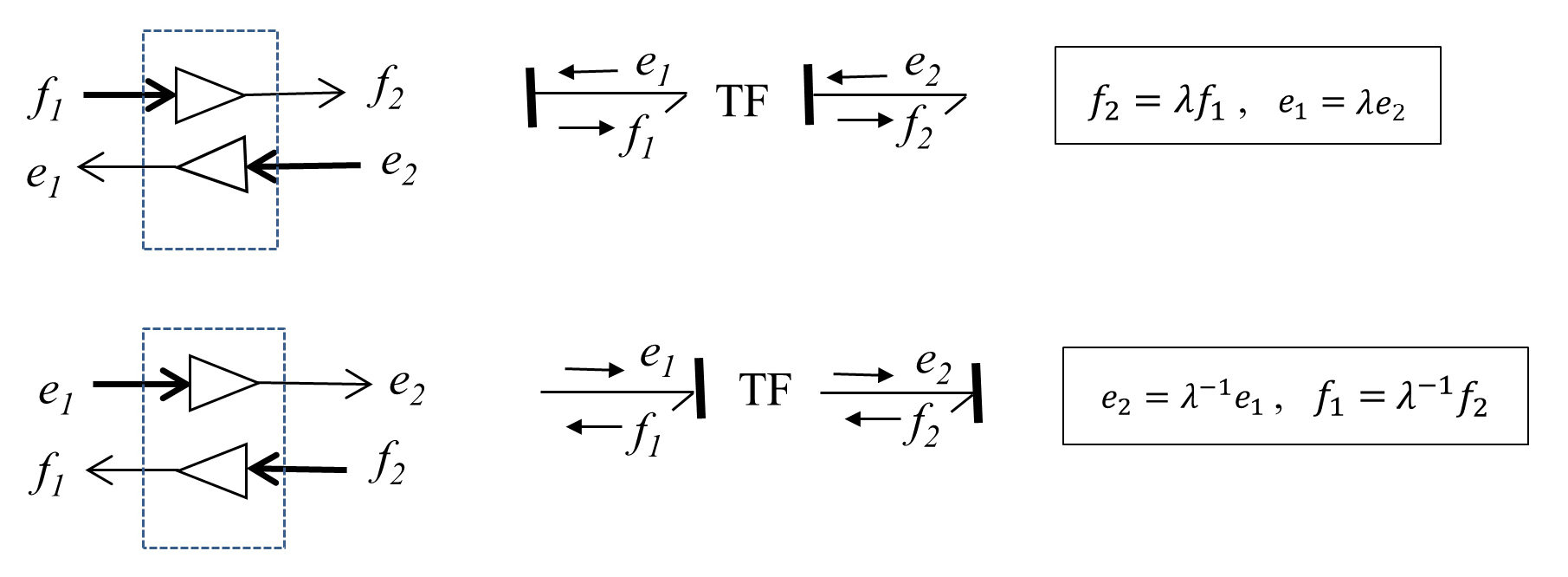 -element with related assigned causalities—inputs are shown with thick arrows
Note that the -element should have only one of the two required causality strokes near it for either cases, as shown in Figure 3‑15.
-element, there should be only one causality stroke close to it and another one away from it. A -element converts flows to flows and efforts to efforts.A gyrator element, , represents the converter that receives a type of physical quantity and delivers a different type after conversion. Examples are a DC motor which converts voltage (effort) to angular velocity (flow) of the rotor or the attached shaft. The reverse operation is that of an electric generator.
As Figure 3‑16 shows, a -element can have one effort and one flow as inputs and, consequently, delivers corresponding flow and effort as outputs. The conversion parameter  should be defined, based on the physical system data. For example, for the case with flow as the input and effort being the output, we can write
  to define . But from energy conservation we have , or the output effort
  . Similarly, for the case with effort as the input and flow being the output, we can write
  , using . But from energy conservation we have , or the output flow
  . These relations constitute the -element equations and are shown for each case where the inputs for the -element are identified with thick arrows in Figure 3‑16.
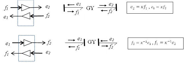
Note that the -element should have both required causality strokes near it or away from it, as shown in Figure 3‑16.
-element, there should be two causality strokes close to it or both away from it. A -element converts flows to efforts and efforts to flows.Now that we have all nine elements of BG method defined, in the following sections we discuss the state variables, their definitions, and relation with integral causality. State variables are key quantities in analyzing engineering system dynamics and behaviour and are a critical part of BG method. A sound understanding of the state variables will help in developing a high level of competency in BG method and its applications to engineering systems.
The main objective of BG models is to derive system equations that describe the behaviour of the system and to follow up by solving these equations for simulation and design purposes.
The system equations may be ODEs of second order or higher. However, when writing these governing system equations in terms of state variables—those variables that uniquely and sufficiently describe the system dynamics—we end up having first-order ODEs, a huge advantage when using numerical/analytical solution methods. In addition, when we extract system equations from the corresponding BG model (see chapter 11), additional algebraic equations are involved; hence, we have a system of differential-algebraic equations (DAEs) that could benefit from having the related ODEs written as first-order equations.
In this section, we define the state variables that relate themselves to the storage elements in BG method i.e., -element and -element. Other BG elements correspond to the algebraic equations of the system DAEs and do not possess state variables of their own.
We now consider the kinetic energy storage element or inertia -element. The energy stored can be written as the integral of power (i.e., effort multiplied by flow) with respect to time,  or as
or as  . But
. But  , the generalized momentum differential/change. Hence,
  , or the energy stored in an inertia element is the integral of flow (e.g., velocity) with respect to momentum as the independent variable. Therefore, a functional form of the type
  is required to perform the integral operation. In other words, the area under the curve of the flow in the
  coordinate system is equal to the energy stored. Recall that, e.g., in mechanical systems, this function (i.e., ), is derived from Newton’s second law, or
  (the parameter is mass or inductance, for example). Therefore, we have
  , or
, or
(3.7) 
Equation (3.7) clearly shows that the energy stored by an -element is uniquely defined by its generalized momentum. Therefore, the momentum of an -element is identified as a state variable of the system.
on .Similarly, we consider the potential energy storage element, or -element. The energy stored can be written as the integral of power with respect to time, or as  . But
. But  , the generalized displacement differential/change. Hence,
  or the energy stored in a -element is the integral of effort (e.g., force) with respect to displacement as the independent variable. Therefore, a functional form of the type
  is required to perform the integral operation. In other words, the area under the curve of as a function of in the
  coordinate system is equal to the energy stored. Recall that, e.g., in mechanical systems, this function (i.e.,
  ) is derived from Hooke’s law, or
  (the parameter is spring compliance or capacitor capacitance, for example). Therefore, we have
  , or
, or
(3.8) 
Equation (3.8) clearly shows that the energy related to a -element is uniquely defined by its generalized displacement. Therefore, the displacement of a -element is identified as a state variable of the system.
-element in the bond graph model is a system state variable, so-called on .
These two state variables ( and ) are key variables when extracting system equations from the corresponding bond graph (see chapter 11). The total number of independent system equations is equal to the total number of state variables, or on and on .
The reader should also note that the assumed governing equations for these two elements (i.e., Newton’s second law for -elements and Hooke’s law for -elements) determine the functional forms of  for an -element and for a -element, respectively. Other constitutive equations: e.g., non-linear relations could be used if desirable, but the uniqueness of energy stored on the and remains for each of these two elements.
The main objective of assigning a causality stroke to an element is to make the element definite in terms of its inputs and outputs (i.e., either effort or flow). Since we have two choices (either effort or flow being the input or the output), the preferred causality is the one that, when assigned, allows the input to the element such that the element-related laws of physics are satisfied and the state variable is concluded as well. For example, if an element receives effort, then it should respond with flow, and the related state variable should be the outcome of the application of the laws of physics to this element. These objectives are met when we use the integral causality strokes for -element and -element. In other words, when the integral of the cause signal is equal to the state variable of the corresponding storage element, then that element is integrally causalled.
In the previous sections (see sections 3.4.1 and 3.4.2), we discussed the preferred causalities for – and – elements as being the integral causality types. Having defined the state variables for – and – elements (see section 3.5), we can expand the discussion on why the integral causality is the preferred one for these elements.
and specifies the assignment of causality strokes for the integral causality is defined such that the integral of input quantity (either effort or flow) for – or -elements result in the corresponding state variable.Recall that generalized momentum is the state variable for an -element. Now, we consider the choice of having the flow or effort as the input for -element according to the causality stroke assignment (see Figure 3‑4). When the effort is selected as the input, we can integrate it (hence, the designation of integral causality for this choice), and get the momentum, i.e., the state variable, as well as the flow for the element response. This is consistent with the -element governing equation (i.e., Newton’s second law). Therefore, having the causality stroke at the port of -element, or the preferred causality assignment (see Figure 3‑4), satisfies all the mathematical requirements and provides the flow as the response and the momentum as the state variable. The whole process is shown in Figure 3‑17. The choice of having flow as the input for -element—the derivative causality—does not fulfill all the objectives mentioned above; hence, it is not preferred. Note that when derivative causality is assigned, Newton’s second law still is satisfied, but the state variable is not explicitly involved.
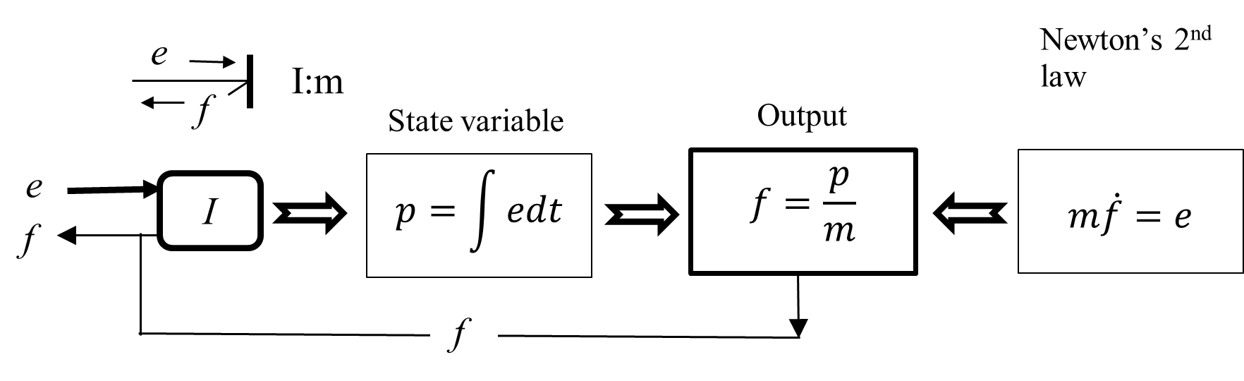 -element with parameter
 Similarly, for a -element, we can have a similar argument. Recall that generalized displacement is the state variable for a -element. Now, we consider the choice of having the flow or effort as the input for -element according to the causality stroke assignment (see Figure 3‑7). When the flow is selected as the input, we can integrate it (hence the designation of integral causality for this choice) and get the displacement, i.e., the state variable, as well as the effort as the element’s response. This is consistent with the -element governing equation, i.e., Hooke’s law. Therefore, having the causality stroke away from the port of -element, or the preferred causality assignment (see Figure 3‑7) satisfies all the mathematical requirements and provides the effort as the response and the displacement as the state variable. The whole process is shown in Figure 3‑18. The choice of having effort as the input for -element—the derivative causality—does not fulfill all the objectives mentioned above; hence, it is not preferred. Note that when derivative causality is assigned Hooke’s law still is satisfied but the state variable is not explicitly involved.
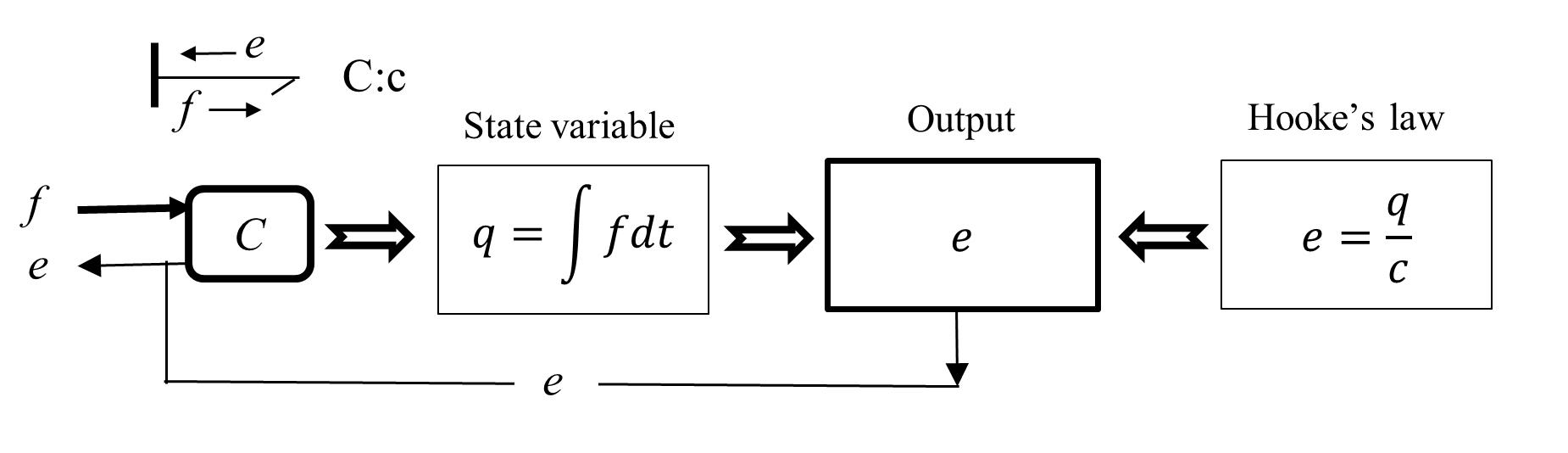 -element with parameter
 Exercises
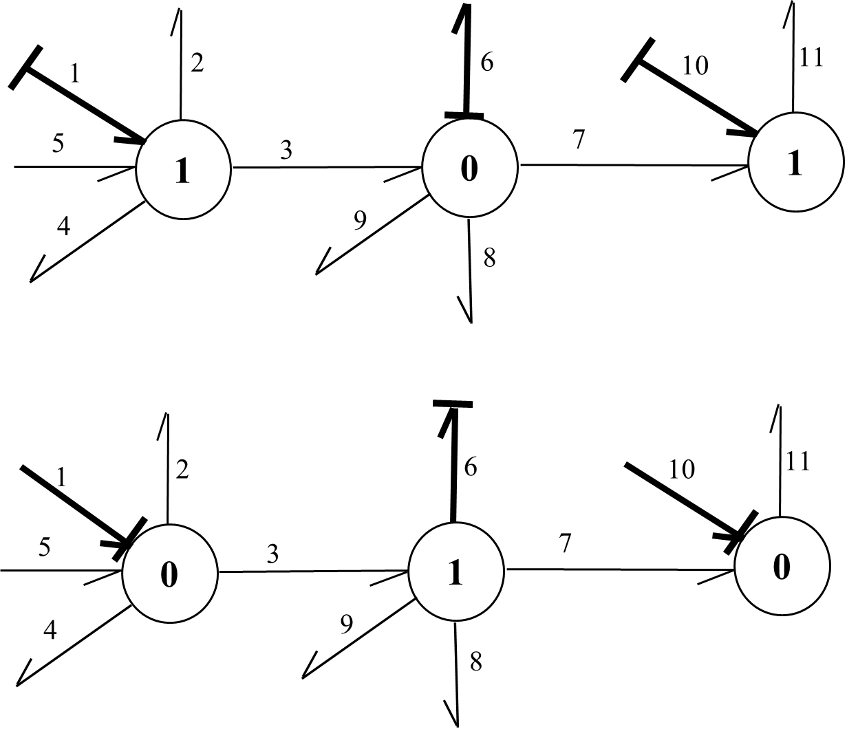
 , as shown in the below sketch. Draw the bond graph model using TF- element along with equation model for each case:
  . Calculate the transformer parameter
  .
. . Calculate the transformer parameter
  and .
and .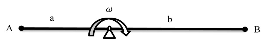

4
To demonstrate applications of BG method, we discuss the procedure for building BG models for physical systems, using the material presented in chapter 3. We use examples related to mechanical systems to establish the guidelines and steps required to build a BG model. In further chapters, we present more worked-out examples for several engineering systems and disciplines, including electrical, hydraulic systems.
As mentioned, BG method can be used to build models for single- and multi-domain physical systems. The building blocks are the nine basic BG elements, including their modulated versions, and causality assignment rules (see section 3.4). A model for any specific system also requires definitions of relevant sign conventions for general displacement and forces. This chapter will discuss the latter and will present some worked-out examples. The following are the steps for building a BG model, in general, including for mechanical, electrical, and hydraulic systems:
and for energy conversionIn further sections, we will demonstrate implementation of the procedure/algorithm mentioned above with some worked-out examples, including power bond direction, causality assignment, and sign convention.
Connecting elements in a BG model with power bonds requires compliance with the direction of energy flow in the physical system. Therefore, the directions of half-arrows are critical. The following guidelines may be helpful:
and ) toward the system, connecting to the adjacent elements., , and )After drawing all power bonds for the model, assign the causality strokes. The next section provides a list of guidelines for causality assignments.
The assignment of causality strokes is a required step in building any BG model. The following steps help with achieving this requirement.
– and – elements. and )-elements that accept neutral causality stroke assignment.If execution of step 5 from the above list cannot be completed, then the BG model contains some specific mathematical properties—algebraic loop or differential/derivative causality (see chapter 11). The application 20-sim automatically assigns the causality strokes with prioritizing integral causalities, and if present, identifies the derivative or algebraic loops causalities in the model with red-colour strokes. In further sections, we will explore these features, with some examples.
A mechanical system consists of mass [kg], spring [N/m], and damper [N.s/m]. The applied force on mass is  . Build a BG model for this system as shown in Figure 4‑1, neglecting friction of the rollers.
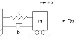
Solution:
DOF = 1 (1D translational motion of one mass) and the required BG elements are: (representing the mass), (representing the spring), (representing the damper), (representing force ) and (representing the wall velocity). Also, we are required to have junctions “1” and “0.”
We draw them as
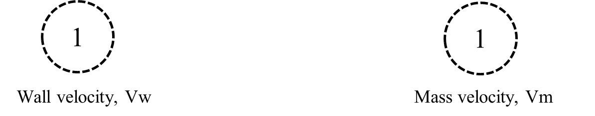
As well, for each junction, it is useful to assign a name related to its representation.
and for mass-velocity junction and inertial element , representing the mass and a representing the applied force  Note that -element should receive power (passive element), and sources send power to the system (active elements).
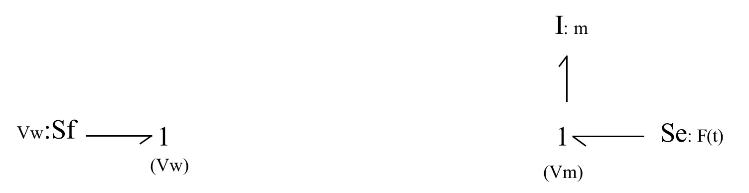
 |, which is represented by 0-junctions. Recall that 0-junction element is a flow summator. According to the power bonds connecting the spring (or damper) to the 0-junction, we can have (
 ) or (
 ), considering the -coordinate as given in Figure 4‑1. Therefore, to specify the associated power bond directions we should define a sign convention. The common practice is to consider the spring (or damper) from the BG model and define either tension force as being positive (+T) or the compression force being positive (+C). For this example, we use the spring displacement/velocity to demonstrate the sign convention. A similar argument applies for the damper’s displacement.
To represent the relative velocity, we add two 0-junctions and – and – elements to the model and use, e.g., (+T) sign convention, as shown below:
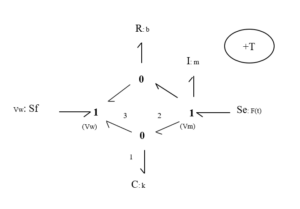 Note that – and – elements are passive and should receive power from the system. After labelling the bonds connecting to the 0-junction associated with the – element, we can write the power balance as
  . But
. But  . Hence,
  , or
, or  where
where  is the spring displacement rate or velocity equal to the relative velocity. Now, to have the displacement of the spring in the + direction, we should have
  or . This implies that the displacement/velocity of the mass should be larger than that of the wall, for the spring is experiencing a positive tension force. Therefore, the spring is under tension and the assigned sign convention (+T) is satisfied, considering the + direction.
Now, if we change the power direction of the bonds connecting to the 0-junction, as shown in the sketch below, we have  , or
, or  ; hence, we have the spring under compression. Therefore, the (+C) sign convention is satisfied. Note that only the power direction of the four bonds associated with the two 0-juctions can change their directions since the rest are associated with source or passive elements and are unique in their directions, as shown below.
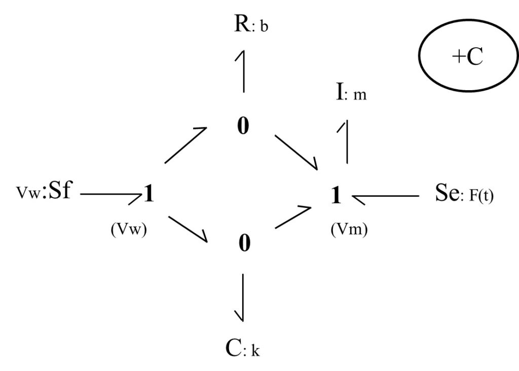 Both sign conventions are legitimate, but only one should be selected and used consistently for building a BG model. We continue, using the BG model with (+T) sign convention.
– and – elements. Recall that integral causalities are preferred for elements (i.e., receives effort) and (i.e., C sends effort). The causality strokes are shown with transvers lines, as shown below.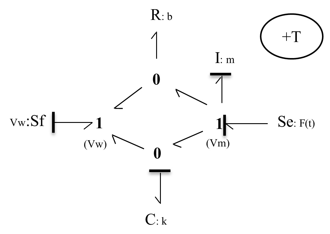
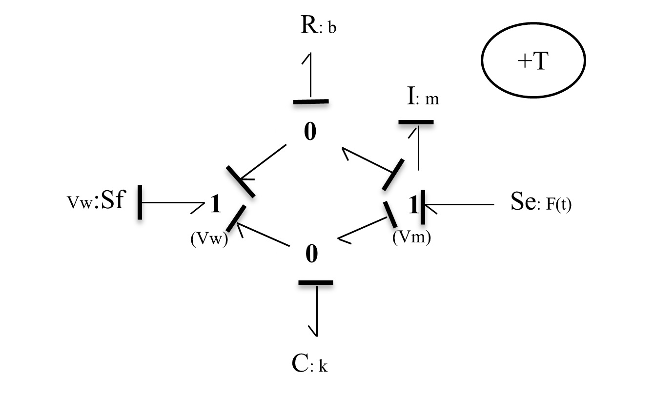
. Therefore, we can combine them into a single 0-junction and share the relative velocity value through a 1-junction element with the – and – elements. This simplification becomes very useful for building large BG models for more complex systems. Figure 4‑3 shows the resulting BG model. Note that the causality strokes should be adjusted after simplifications are made.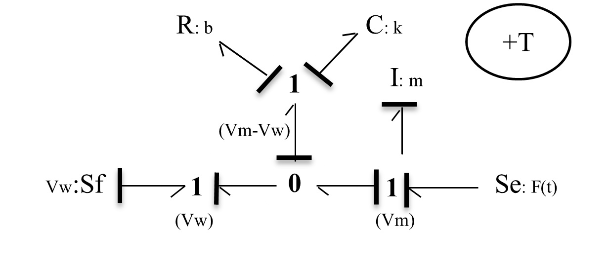
Build the BG model for the mechanical system as shown in Figure 4-4. Consider the (+C) to be the sign convention for internal forces.
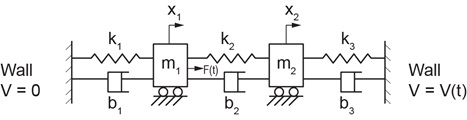
Solution:
This system has two DOF and four distinct velocity points, corresponding to mass and and the two walls. Therefore, we lay out four 1-junctions to represent them in the model. The remaining required BG elements are , , , , , and 1- and 0- junctions.
We follow the same guidelines demonstrated in the previous example (see section 4.3) and build the BG model as shown in Figure 4-5.
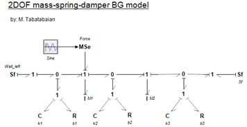
The reader is encouraged to build this BG model and to compare the results with those provided in Figure 4-5. The 20-sim BG model and a screen recording are available as companion resources describing the process to build the equation model and typical results for this example.
Build the BG model for the mechanical system as shown in Figure 4-6. Consider the (+C) to be the sign convention for internal forces.
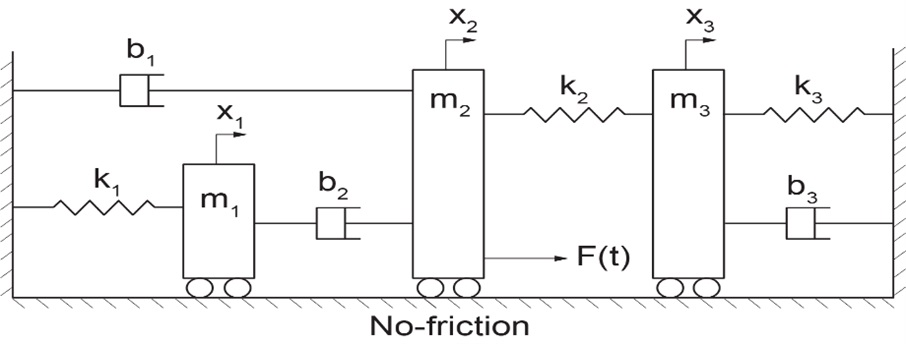
Solution:
This system has three DOF and five distinct velocity points corresponding to mass , , and and the two walls. Therefore, we lay out five 1-junctions to represent them in the model. The remaining required BG elements are , , , , , and 1- and 0-junctions.
We follow the same guidelines demonstrated in the previous example (see section 4.3) and build the BG model, as shown in Figure 4-7.
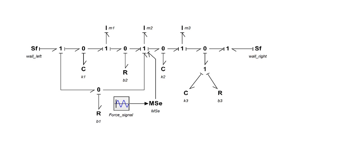
The reader is encouraged to build this BG model and compare the results with those provided in Figure 4-7. The 20-sim BG model and a screen recording are available as companion resources describing the process to build the equation model and typical results for this example.
As mentioned previously (see section 3.2), one of the advantages of BG modelling method is that a BG model allows us to gain insights by visual inspection of the BG model. This can be achieved by drawing the streams of efforts (kinetics) and flows (kinematics) for a BG model.
In this example, we use the results from the example given in section 4.3 to demonstrate this property by explicitly drawing the effort and flow associated with each power bond in the model. First, we look at the kinetics of the system by drawing the efforts, as shown in Figure 4-8. As shown, the efforts/forces associated with the spring  and dumper
  are collected as force and transferred to the mass in addition to the applied force shown as
  . Clearly, the wall receives the collected force
  .
.
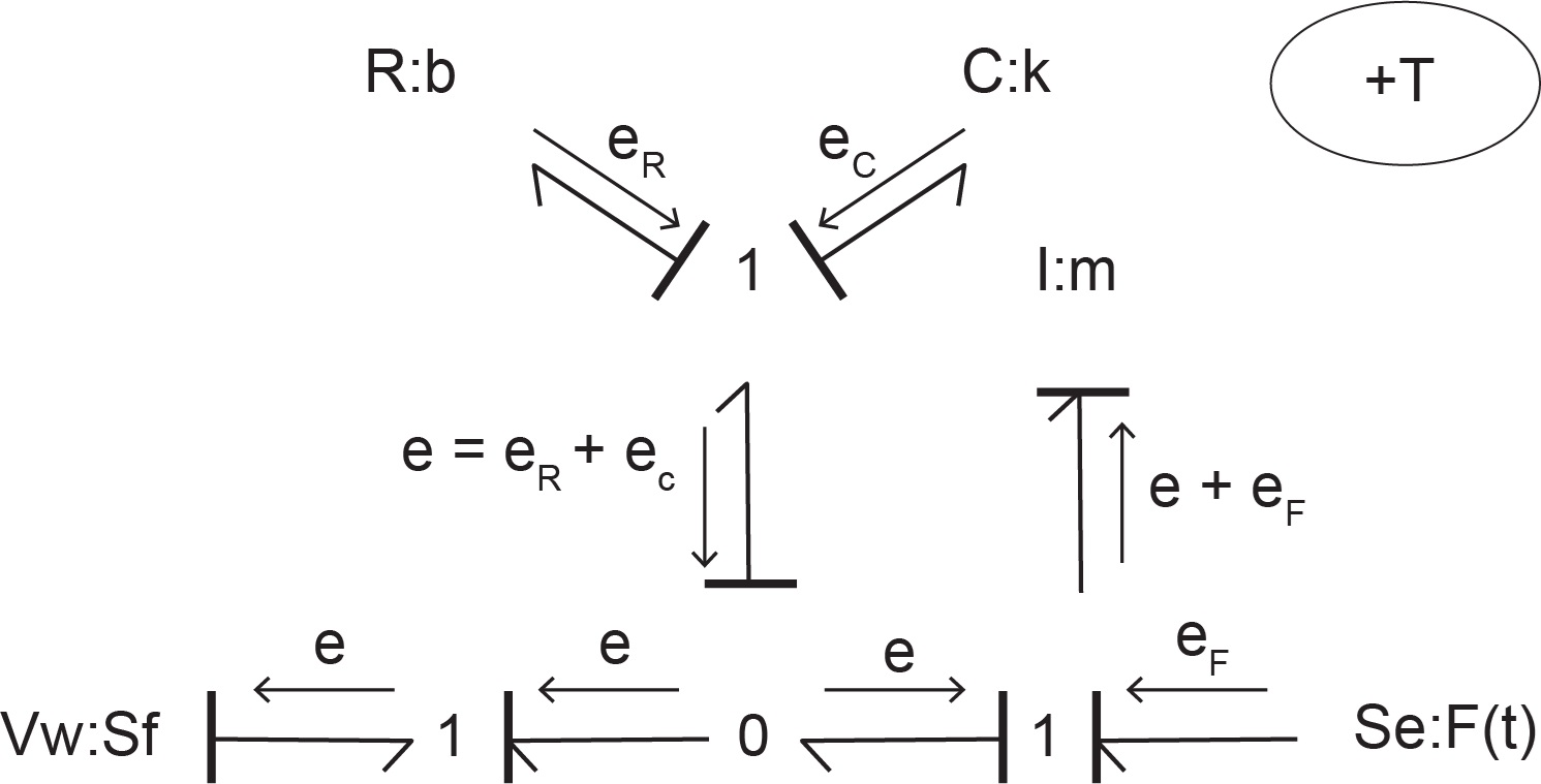
Similarly, by drawing the flows, as shown in Figure 4-9 the kinematics of the system can be visualized. As shown, the flows/velocities associated with the mass  and wall
  are collected as velocity and transferred to the spring and damper. Clearly, these elements receive the relative velocity
  due to the motion of mass and the wall (if stationary,
  ).
).
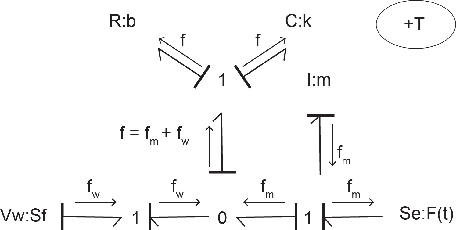
Considering BG—our focus in this textbook—as the modelling method, once we have the corresponding BG model, we can proceed to simulation, and hence, design of a system. One can take two approaches to perform this task: traditional or modern. As mentioned, the main objective of modelling and simulation is to help with more effective design of the systems in terms of their cost, function, material consumption, etc. Therefore, any modelling method, including bond graph, should result in a mathematical model consisting of the systems’ equations. The solution of the equations can be used for system simulation and analysis to support effective system design. In the following sections, we briefly describe possible approaches and the reason for choosing the modern approach over the more traditional one.
Once the BG model is available for a system, we can derive/extract the system equations from the BG model—usually a laborious task—and then using numerical methods, we can obtain their solutions. This task is usually achieved with the help of computer programs (usually developed from scratch) based on a selected numerical method. This approach, along with both its system equation extraction and especially the computer coding, is limited in practical application, being specific from one problem to another one, and is laboriously time consuming. Figure 4-10 shows the major steps of the traditional approach.
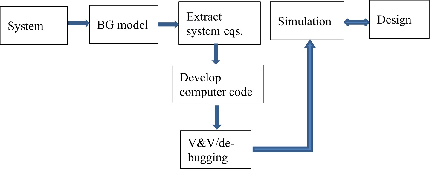
In practice, it is inefficient to develop computer codes for each specific design: the amount of person power, computer power, and other resources become overwhelming for the fast-paced engineering design needs of today’s industries. Therefore, a huge effort has been made to develop commercially available software tools to help meet these objectives and to make the whole process of system design more effective, economically viable, and efficient.
Alternatively—or rather, preferably—the modern approach in engineering and system design employs related software tools. These tools provide opportunities to perform systems simulation immediately after obtaining the BG model. The software tool that we introduce and use in this textbook, 20-sim, helps with extracting the system equations from the BG model seamlessly and provides facilities for system simulation and parametric analysis. This modern approach is more effective in engineering practice and provides more and quicker insights into engineering systems design. In addition, the modern approach helps to respond more effectively to the fast-paced engineering demands in industry and is recommended for engineers in practice. Figure 4-11 shows the major steps of the modern approach. Note that verification and validation should be considered in the modelling step as well.
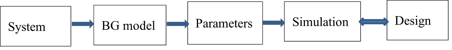
In the next section, we introduce the 20-sim software package with a focus on bond graph modelling, simulation, and time and frequency analysis for engineering systems and design. In further sections, we use 20-sim to build BG models and their simulations and to study their dynamical behaviour.
Exercises
5
In this chapter, we introduce the engineering software tool 20-sim, focusing on its BG modelling and simulation facilities. Originally developed in the Netherlands at the University of Twente and released in 1995, 20-sim was the first commercially released software package for bond graph modelling. 20-sim was further developed and currently is available through Controllab Products [3].
An advanced modelling and simulation software tool, 20-sim uses Microsoft Windows™ operating system. 20-sim enables users to model the behaviour of systems, such as mechanical, electrical, hydraulic, thermal, or a combination of these systems (i.e., multi-domain systems). Below is a list of 20-sim’s modelling and simulation tools. The first four items in the list are the main tools:
20-sim allows users create models graphically, similar to drawing an engineering sketch. With these models you can simulate and analyze the behaviour of single-domain and multi-domain dynamic systems and create control systems. One can even generate C-code and run this code on hardware for rapid prototyping and hardware-in-the-loop (HIL) simulation.
20-sim has two main window interfaces: Editor and Simulator, shown in Figure 5‑1 and Figure 5‑2, respectively. To open the Simulator window from the keyboard, select Ctrl + R. To open the Simulator window from the Editor window, choose Tools > Simulator.
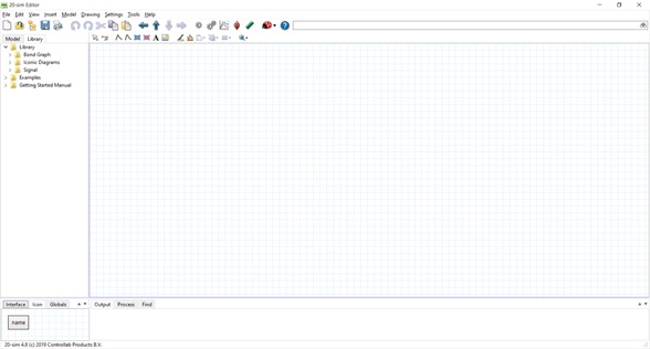
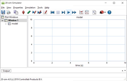
As described in the manual Getting started with 20-sim 4.8, the Editor consists of four parts:
Here is a video guiding the reader through the features of 20-sim:
More information about using 20-sim is available at 20-sim webhelp and at 20-sim Help Manuals.
Figure 5‑3 shows the main steps for system design. In further sections, we will follow these steps with several worked-out examples to demonstrate the application of this process.
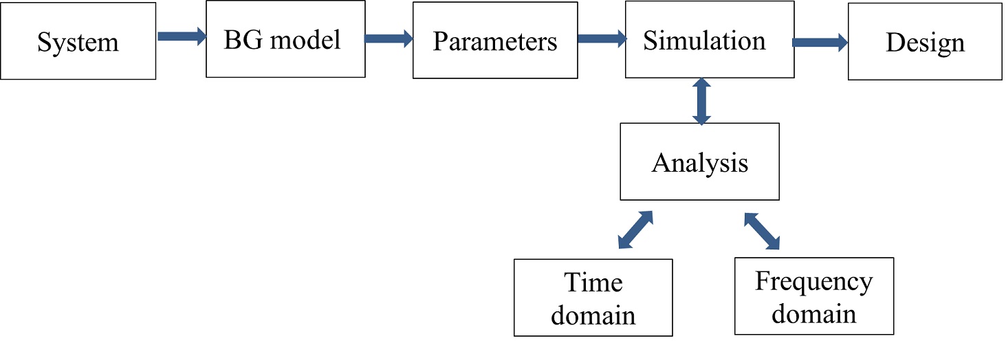
To demonstrate 20-sim application, using the data provided in Table 5‑1, we build a BG model of a car seat. The car seat system schematic is shown in Figure 5‑4. Consider the (+C) to be the sign convention for internal forces.
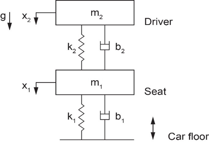
| Component/element | Value | Unit |
| Mass, | 27 | kg |
| Mass, | 80 | kg |
| Spring, | 1800 | N/m |
| Spring, | 19 x 104 | N/m |
| Damper, | 400 | N.s/m |
| Damper, | 900 | N.s/m |
Car floor speed,  | signal | step-function |
Solution:
Here are two videos showing how to build and run the model for this example in 20-sim:
Launch 20-sim and follow the solution steps provided in the videos. Figure 5‑5 shows the resulting BG model.
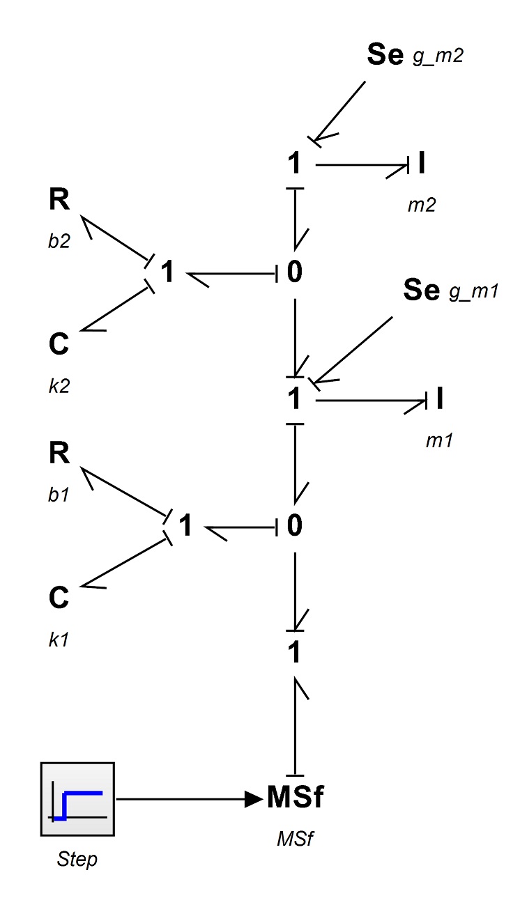
To demonstrate 20-sim, we build a BG model of a cart carrying a load. Consider the (+C) to be the sign convention for internal forces.
Table 5‑2 shows the data for the system components. Figure 5‑6 shows the cart system schematic.
| Component/element | Value | Unit |
| Mass, | 40 | kg |
| Mass, | 20 | kg |
| Spring, | 2000 | N/m |
| Spring, | 1500 | N/m |
| Damper, | 400 | N.s/m |
| Damper, | 900 | N.s/m |
| Force, | signal | sinusoidal |
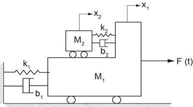
Solution:
The process for building a BG model and related simulation for this example is given through a screen recording that guides the readers through the whole process. Launch 20-sim, and to build and run the 20-sim model for this example, follow the solution steps provided in the following video:
Figure 5‑7 shows the resulting BG model.
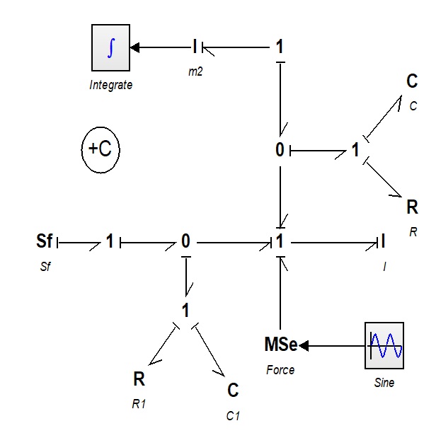
Exercises
Run the model for simulation and create and report typical graphs.
Run the model for simulation and create and report typical graphs.
6
In the previous chapters, we established concepts such as the basic elements of bond graph method and the algorithm for building BG models. We now continue with more worked-out examples for selected complex mechanical systems. These systems may have many components, involve many degrees of freedom, and exhibit translational and rotational motions in one-dimensional (1D) or two-dimensional (2D) space. So far, we have used translational mechanical systems and demonstrated how to build their related BG models (see chapters 4 and 5). In this chapter, we expand the discussion to rotational mechanical systems with rotational and/or 2D/plane rigid-body motions, including their related BG model examples. First, we establish the theories and related equations and then use those for building the BG models.
A mechanical system may consist of rotational components, e.g., shafts, discs, gears, pulleys, and levers. The generalized BG elements and relations apply to the motion of rotational components in a similar way that the translational motion was treated; i.e., they are analogous (see Table 3‑1). In other words, rotation angle is equivalent to the generalized displacement , angular velocity  to the flow , and torque to the effort . The polar moment of inertia
  is represented by -element, the shaft by -element, and bearing by -element. The generalized momentum is the integral of with respect to time. Therefore, we can write

where  is the rotational momentum or so-called angular momentum. Using the constitutive relations, for an -element we have
  or
or  , for a -element we have
  or,
or,  where represents the torsional compliance or inverse of torsional stiffness
  ,
,  . Similarly, for an -element we have or
  where
where  is the friction of the torsional bearing. The energy associated with storage elements can be written using Equations (3.7) and (3.8), or for elements and , as
  and
and  , respectively. One advantage of bond graph method is its analogous applicability to different domains using the common constitutive relations, as described above for rotational motion.
Table 6‑1 shows typical rotational components.
| -element (bearings) | -element (shaft) | -element (disc) | -element (gears) | -element (gyrator) |
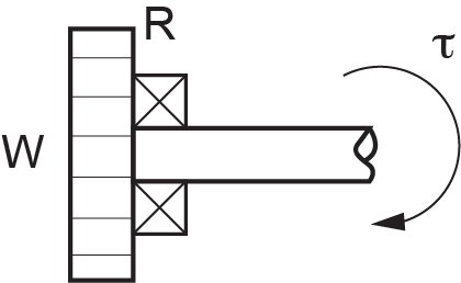 | 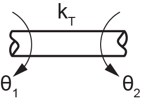 | 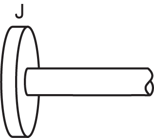 | 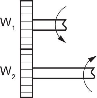 | 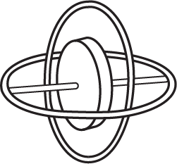 |
The components of mechanical systems that we considered so far are assumed as point masses. In other words, they are point elements but can have motions either in translation and/or rotation. However, two-dimensional components such as rigid plates, car chassis, and thin rods can have relative 2D motion and cannot be treated as point elements.
In general, a 3D solid component/body has six degrees of freedom; i.e., its centre of mass can move in three translational directions and through three associated rotational angles. In many mechanical systems, however, we can assume components as two-dimensional planes with negligible deformations, or as 2D rigid bodies having three degrees of freedom: two in-plane translations and one rotation about the perpendicular axis to the plane of motion.
Building a BG model requires transforming the velocities and angular velocities associated with the rigid plane and making them available to the contact points with other components of the system. For example, a car’s chassis moving forward on a wavy road may experience rotations like pitch and roll (i.e., rotations about the axes parallel to the ground) in addition to translational motion. Considering the chassis as a 2D rigid body, we need to know how the linear and angular velocities are transmitted to the suspensions connecting to it.
We present here an analysis of 2D rigid-body motion, with focus on applications to BG modelling. For further readings on this topic, consult with available references [13], [18], [20], [23].
The general motion of a 2D rigid body can be decomposed into translation of the whole body and a rotation about a fixed point of the body. This is the result of the principle of superposition and can be shown using the geometry of the motion. As Figure 6‑1 shows, we assume a rigid body going through a planar motion with reference to a fixed coordinate system . We identify a line/vector on the body connecting two arbitrarily selected points A and B, with point B taken as a reference, usually the centre of mass. We then capture a picture of the body at a later time,  during its motion, and find out the line BA in its new orientation and position, as shown in the sketch on the right in Figure 6‑1. Since the body does not deform, the length of the line BA (or the magnitude of vector
  ) remains constant. Using this property, we can draw a circle with its centre at the new position of point B and radius of BA. Then, we draw the radial line BA’ parallel to the line BA at its initial position. To orient BA’ according to the new position of BA, we then rotate BA’ about point B through angle
  , where
  is the magnitude of the angular velocity vector of the rigid body, perpendicular to the plane of motion. Consequently, we can claim that original point A is translated (not rotated) by the velocity of point B,
  from its initial position to a new position A’ and subsequently rotated about point B by angle to orient in its final new position of point A. The initial position of point A is arbitrarily selected; therefore, the argument equally applies to all points of the rigid body.
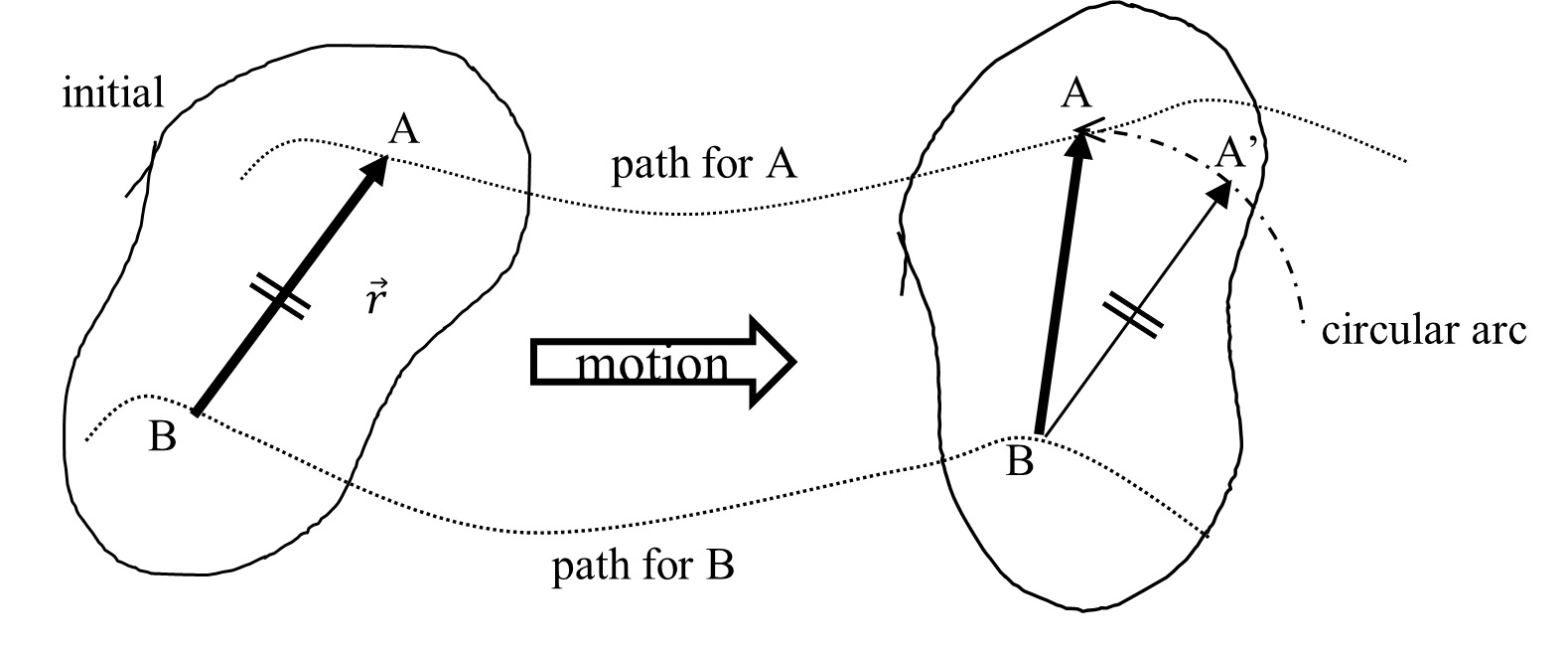
Mathematically, we can write  . The relative velocity
  is the tangential velocity due to rotation and can be written as
  . Therefore,
  . Therefore, we can write the velocity components of point A resulted from rigid-body motion as
(6.1) 
But  and
and  where, is the angle between vector
  and positive direction of -axis. After substituting, we get
(6.2) 
We can use Equations (6.2) for large rotations. However, for small rotations (i.e.,  ), we can linearize these relations by substituting for
  and
and  , or
, or
(6.3) 
For example, for a car chassis, the front and rear ends are moving with the same speed as that of the centre of mass, and their velocities in the vertical direction are the algebraic sum of the vertical speed and that of due to the pitch rotation (i.e., rotation about the axis parallel to the ground and perpendicular to the direction of the motion). See the example in section 6.7.
In the following sections, we present examples of several mechanical systems along with their BG models.
The sketch in Figure 6‑2 shows a system composed of four gears, three shafts, six bearings, and two discs.
For gears, use velocity ratio,  equal to the inverse ratio of the number of teeth, or gears’ diameters, given by
  . Angular velocity of gears is represented by the symbol . System data is given in Table 6‑2.

Solution:
This system has six distinct angular velocities related to gears and discs. The torsional shafts are potential energy storages, and the torsional inertia are kinetic energy storages. The BG elements required are , , , , , and 1- and 0-junctions.
The following video shows how to build and run the model for this example in 20-sim.
The resulted BG models are shown in Figure 6‑3 and Figure 6‑4.
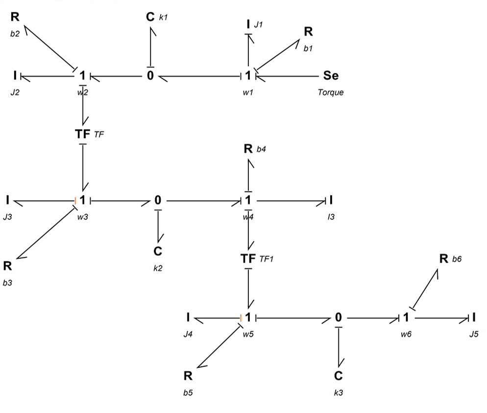
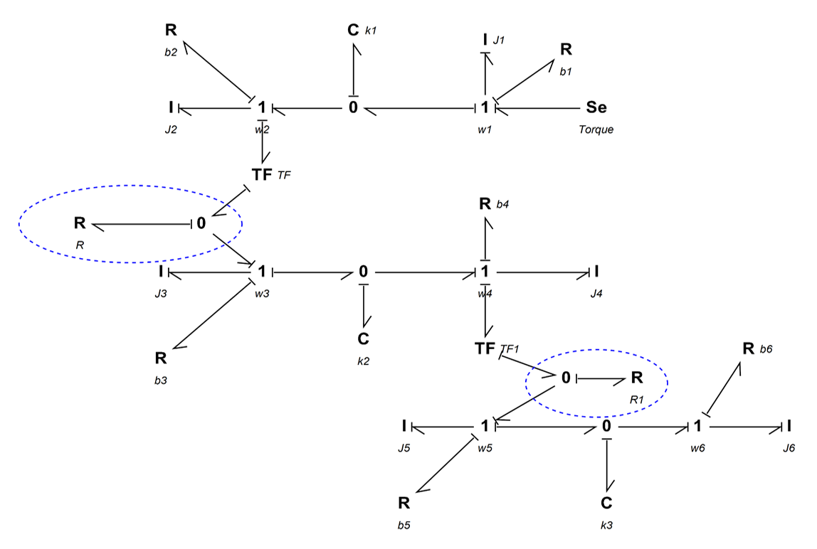
Figure 6‑5 shows a double rack-and-pinion mechanical system. Build a BG model for this system using 20-sim. A torque is applied on the disc connected to the two shafts.
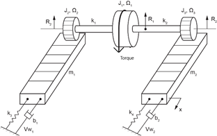
The following video shows how to build and run the model for this example in 20-sim.
Figure 6‑6 shows the BG model for this system.
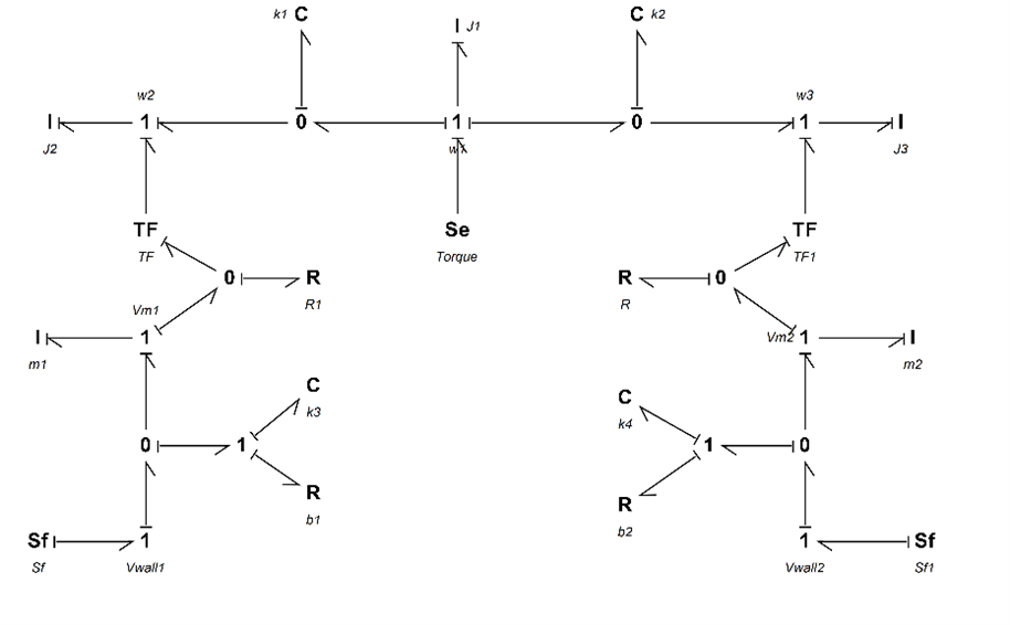
Figure 6‑7 show a mass-spring-damper system on an inclined plane. Build a BG model for this system using 20-sim. Build a BG model for this system using 20-sim.
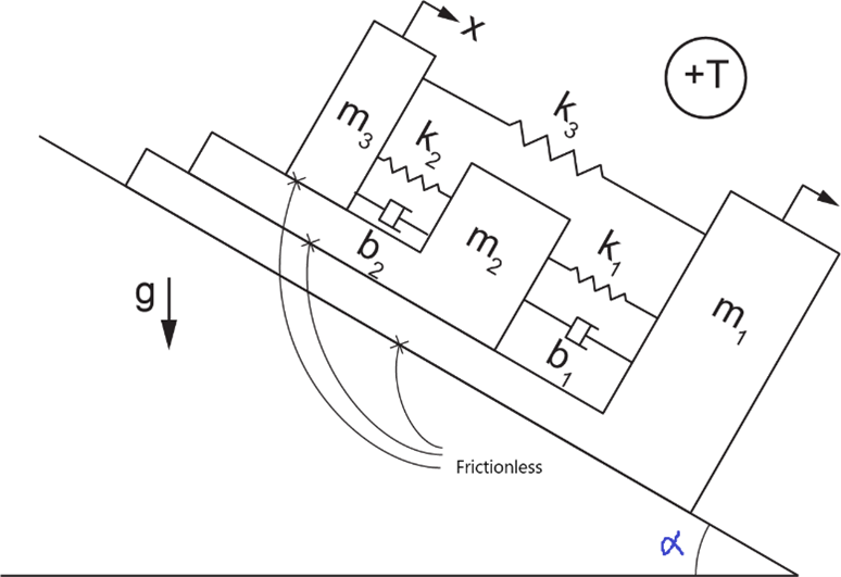
The following video shows how to build and run the model for this example in 20-sim.
Figure 6‑8 shows the BG model for this system.
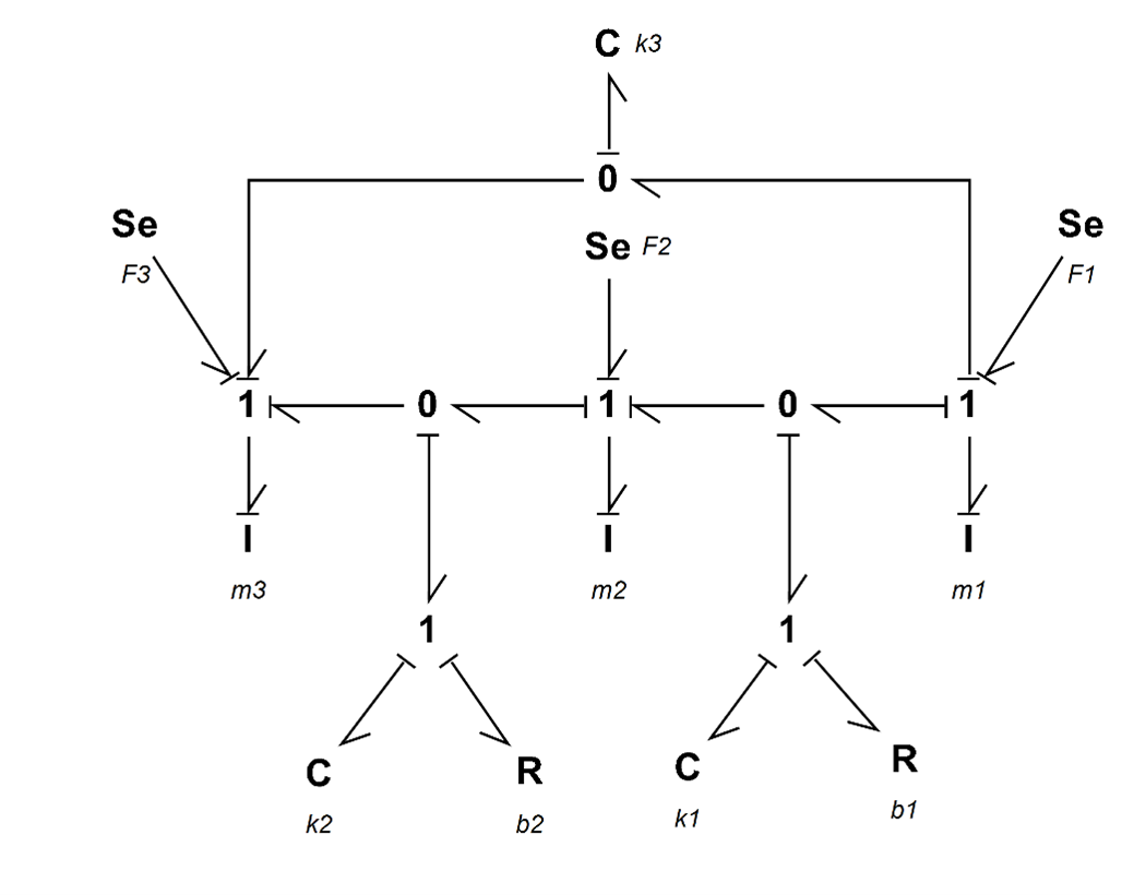
In this example, we demonstrate how to build a BG model for a half-car model as shown in Figure 6‑9. The chassis of the car is modelled as a rigid body with two degrees of freedom. The vertical displacement of the centre of mass is the heave, and its angular velocity is the pitch rate. In the BG model, transformer elements are used to transfer the front and rear velocities to the corresponding connecting points between the suspensions and the chassis. The suspension are modelled as spring-dampers and the tires as mass-spring subsystems.
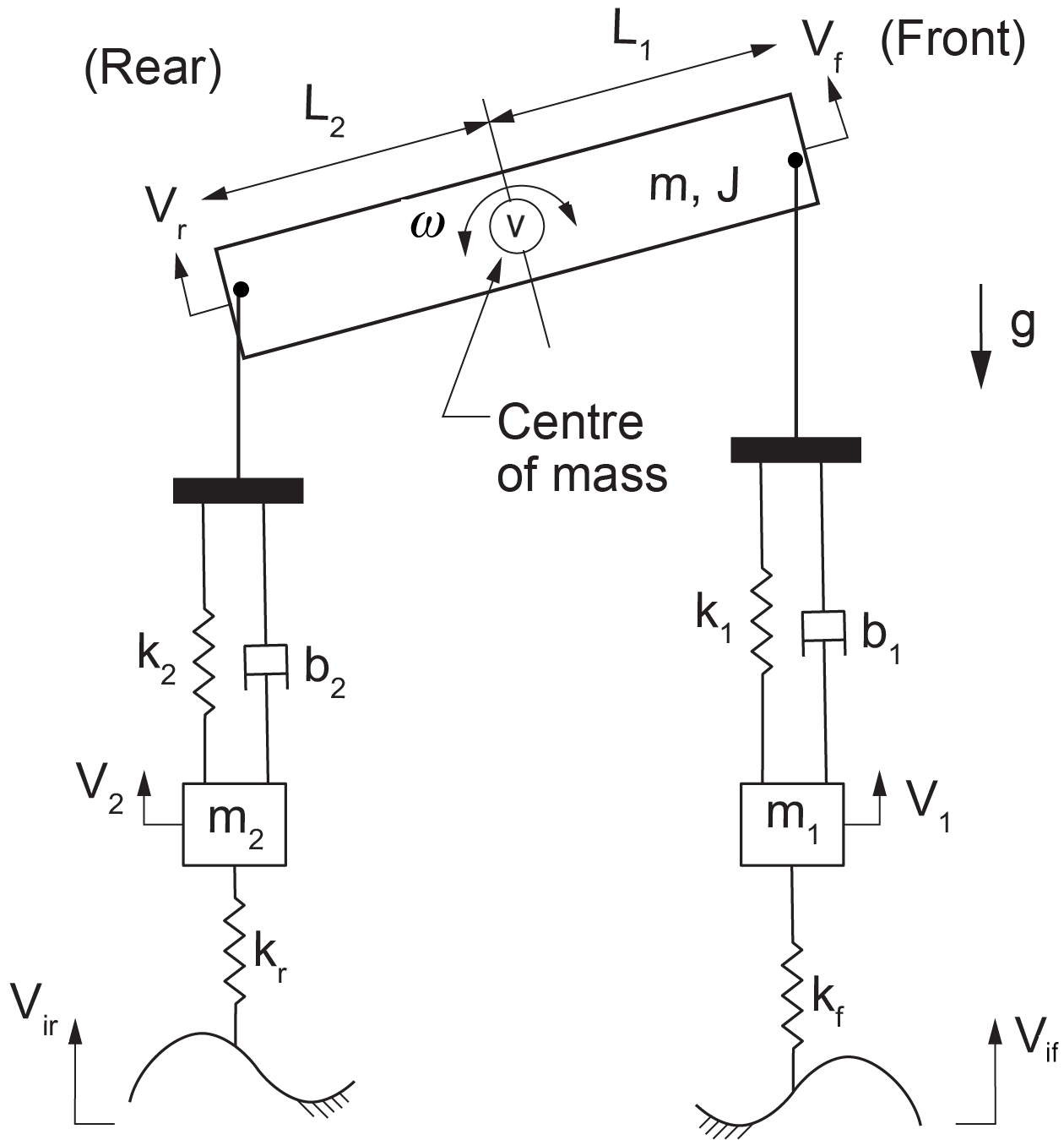
Below are two videos (parts 1 and 2) showing how to build and run the model for this example in 20-sim, including the implementation of the BG transformer element and the setup of the equation model.
Watch the videos and practice building the model on your own, with modified parameters and input signals.
Figure 6‑10 shows the corresponding BG model. The compression force is considered to be positive.
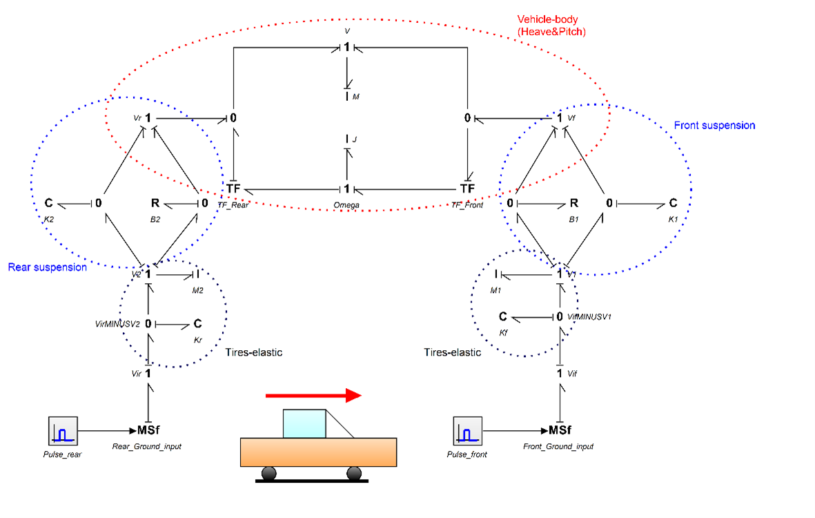
In this example, we demonstrate how to build a BG model for the mechanical system shown in Figure 6‑11. The lever is represented with a -element.
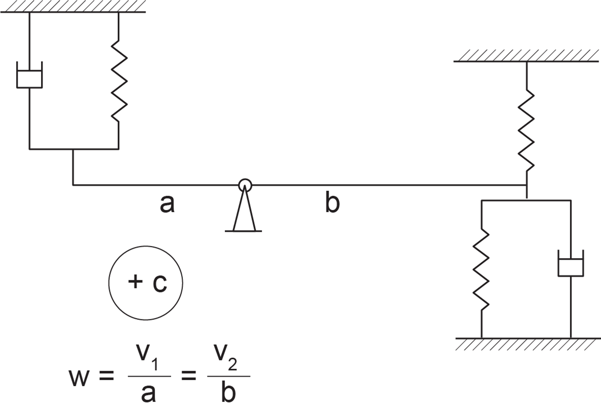
Below are two videos (parts 1 and 2) showing how to build and run the model for this example in 20-sim, including the implementation of the BG transformer element and the setup of the equation model.
For this example we discuss and demonstrate how to build a BG model for the mechanical system as shown in Figure 6‑12. The lever is represented with a -element.
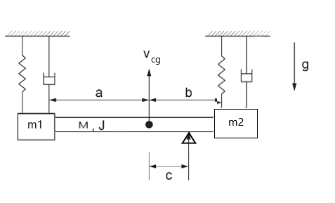
Below are two videos (parts 1 and 2) showing how to build and run the model for this example in 20-sim, including the implementation of the BG transformer element and the setup of the equation model.
In this example, we demonstrate how to build a BG model for a mechanical system consisting of two moving masses attached to a rod, as shown in Figure 6‑13. The rod can rotate as a lever and is represented with a -element.
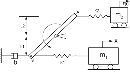
The following video shows how to build and run the model for this example in 20-sim.
In this example, we demonstrate how to build a BG model for a mechanical system consisting of two pulleys and three masses, as shown in Figure 6‑14.
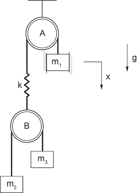
The video below shows how to build and run the model for this example in 20-sim.
Exercises
 ,
,  (kg),
(kg),  ,
,  (m),
(m),  (kg.m2/rad),
  ,
,  ,
,  (kN/m),
  ,
,  (kN.s/m)
  ,
,  , and spring
  . Consider the floor velocity input as a pulse signal with start time of 3 sec., stop time of 4.5 sec., and amplitude of 10 cm. Compression forces are considered to be positive (+C). Gravity direction and positive displacements are shown in the sketch.
| Masses (kg) |  |  |  |  |  | — |
| Springs (N/m) |  |  |  |  |  |  |
| Dampers (N.s/m) |  |  |  |  |  |  |
7
An electrical system may consist of components such as resistors, inductors, capacitors, transformers, and batteries/source. The generalized BG elements and relations apply to the analysis of dynamics of electrical systems and components in a similar way that the mechanical components were treated; i.e., they are analogous (see Table 3-1). In other words, electric charge  is equivalent to the generalized displacement , electrical current to
  to the flow , and voltage to the effort . The inductor (with inductance ) is analogous to point mass and is represented by -element; the capacitor (with capacitance ) is analogous to a mechanical spring and is represented by -element; and resistor (with resistance ) is analogous to mechanical damper and is represented by -element. The generalized momentum
  or flux linkage is the integral of with respect to time. Therefore, we can write

Using the constitutive relations, for an -element we have  or
or  , and for a C-element we have or
  . Similarly, for an R-element we have or
  . The energy associated with storage elements can be written using Equations (3.7) and (3.8), or for elements I and C, as
  and
and  , respectively. An advantage of the bond graph method is its analogous applicability to different domains using the common constitutive relations, as described above for electrical systems.
The analogy between mechanical and electrical systems can be summarized as follows:
In other words, the relations of efforts and flows are swapped according to the type of the physical system between mechanical and electrical systems.

Table 7-1 shows typical components for resistor/, capacitor/, Inductor/, Transformer/, Electric motor/.
| -Element (resistor) | -Element (capacitor) | -Element (inductor) | -Element (transformer) | -Element (electric motor) |
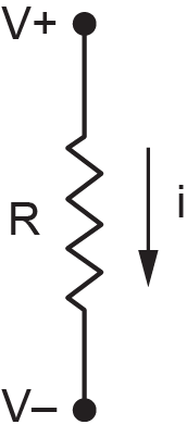 |  | 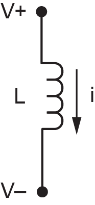 | 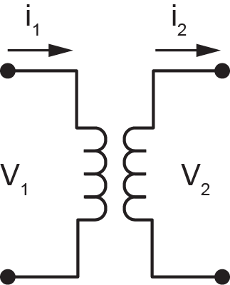 | 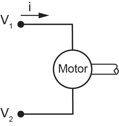 |
Like mechanical systems, for which we defined +C and +T sign convention for internal forces, we require to define a sign convention for electrical systems. It is customary to use the passive sign convention (PSC) for defining the direction of electrical current ( ) passing through the elements of an electrical circuit. The background for the PSC is to have power being positive when absorbed by passive elements, e.g., -, -, and -elements in BG method. Therefore, for a typical passive element, by definition, the electrical current is considered as being positive when input into the element from its higher-voltage node (i.e., positive voltage/
 ) and output from the relatively lower-voltage node (i.e., negative voltage/
 ). Otherwise, the current is negative. See Figure 7‑1.
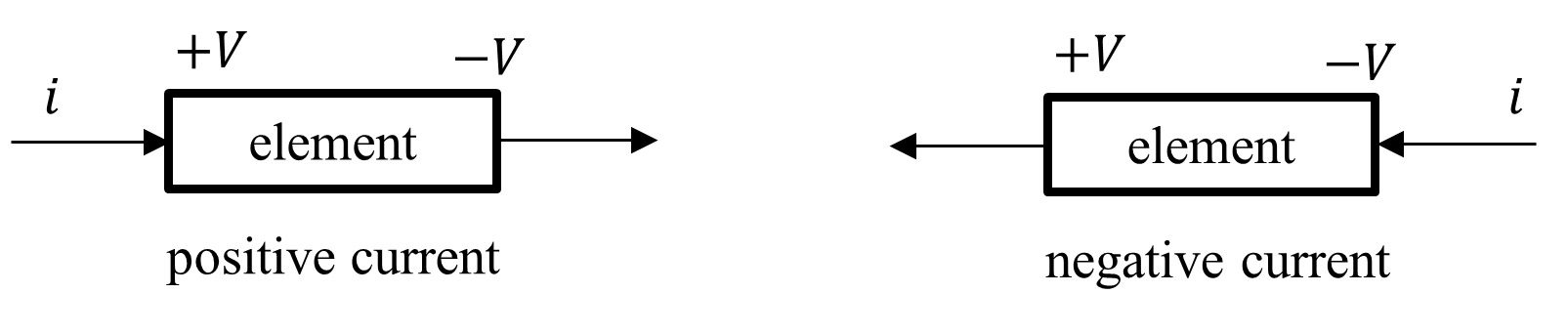
Using the PSC, we have power defined positive for positive current and negative for negative current, or  when
when  and
and  ; hence, power is absorbed by the element. Otherwise, power is generated, when
  when and
  . Figure 7‑2 shows the electrical power sign convention for passive elements (, , ) and active elements (voltage and current sources).
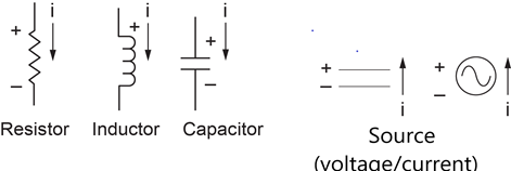
In the next section, we use the PSC for defining the current and voltage signs and discuss the step-by-step procedure for building BG models for electrical systems.
As mentioned in chapter 4, the general guidelines for drawing BG model can be applied to electrical systems along with causality assignment rules. For electrical systems, we follow these guidelines, along with Kirchhoff’s circuit laws [24] and the PSC for building their BG models, as described in the following steps:
 ) for each element in the electrical circuit.-element for capacitors, -element for resistors, -element for inductors, for voltage, and for current sources.-element for electrical transformers and -element for electric motors.
The above steps are based on KVL, and the process starts with assigning 0-junctions for each distinct voltage node. It is also possible to start with KCL and assign 1-junctions for the current in each closed-circuit loop and use 0-junctions in between for distribution of the current to corresponding circuit loops. The latter will result in a more simplified BG model and is recommended for complex circuits that involve several electric loops. In practice, we sometimes use a combination of these two approaches for building BG model for electrical systems.
In the following sections, we demonstrate the application of the procedure discussed above, with some worked-out examples.
Figure 7‑3 shows an RCL circuit consisting of a resistor, a capacitor, and an inductor connected in series. To build the BG model, we apply the PSC and use the procedure listed in section 7.3. The four nodes identified by solid circles have distinct voltages. Therefore, four 0-junctions are assigned at the four corners of the circuit. For voltage drop across each element, we assign 1-juction and connect it to the corresponding element with a power bond. Note that the current direction in the circuit is consistent with the PSC convention. The resulting BG model is shown in Figure 7‑4 after being simplified with deleted ground-connecting bonds shown in the dashed circle. Alternatively, we can simplify the BG model and use a 1-juction for the current in the circuit loop according to KCL. In other words, the electrical current flowing through all elements should be identical. The resulting simplified BG model is shown in Figure 7‑5.
It is useful to discuss the analogy between the RCL circuit and mechanical mass-spring-damper systems (see Figure 4‑1) and their identical BG model. Assuming a ground connection for the circuit is analogous to a wall with zero velocity for the mass-spring-damper system, the current through the inductor is analogous to the velocity of the mass. The same current flows through the resistor and the capacitors, analogous to the velocity of the spring and damper components. Therefore, the simplified BG model (see Figure 7‑5) is identical for both electrical and mechanical systems. In other words, the BG model is identical to the one for a mass-spring-damper connected in parallel.
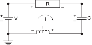
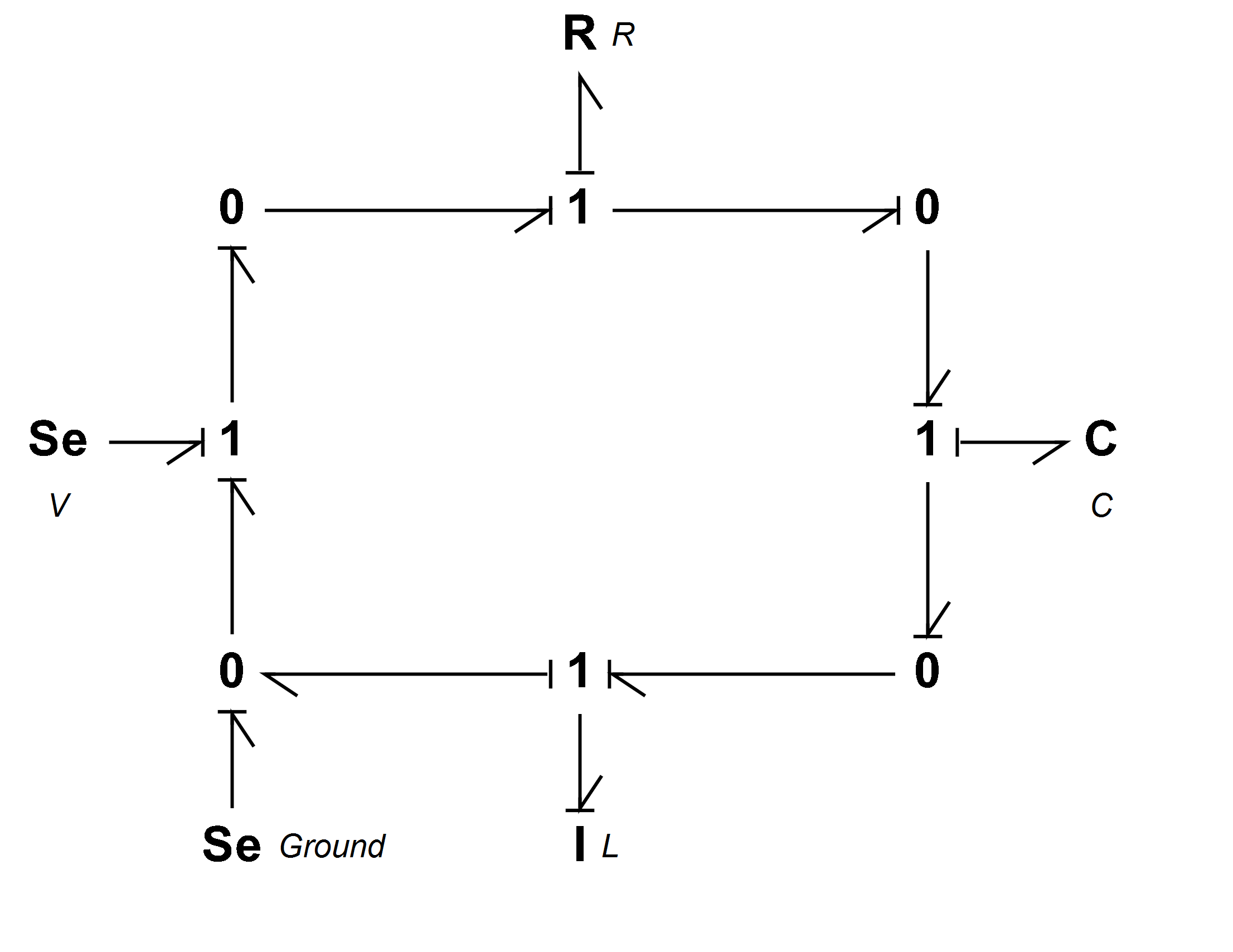
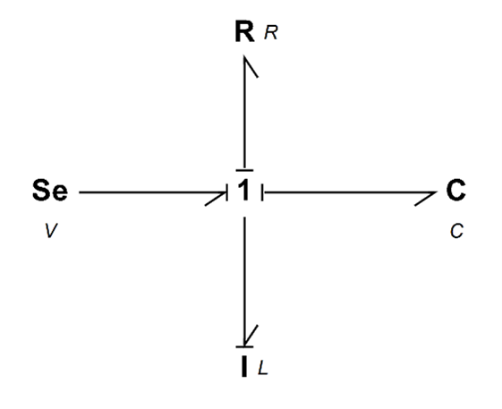
Figure 7‑6 shows an RCL circuit consisting of two inductors, a resistor, and a capacitor connected in parallel. We use the KCL approach to build the BG model for this example. Because the voltages across all components are identical, we can, using power bonds, apply a 0-junction (i.e., voltage equalizer) and connect the , , and components to it. This can be obtained by simplifying the BG model shown in Figure 7‑7.
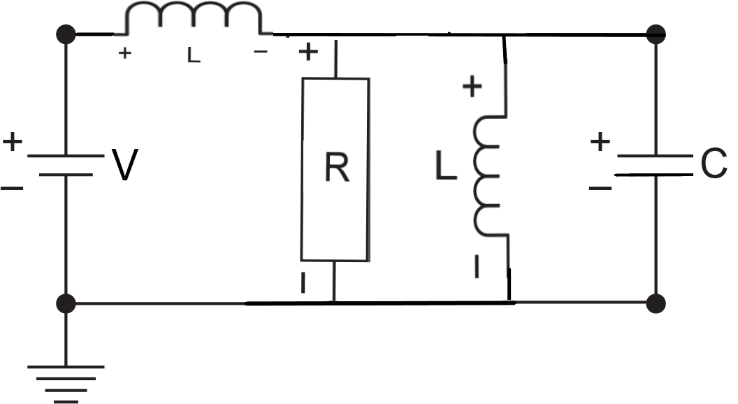
The following video shows how to build and run the model for this example in 20-sim.
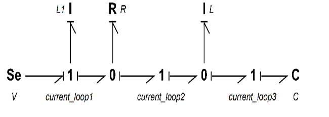
Figure 7‑8 shows an RCL two-loop circuit consisting of resistors, inductors, and a capacitor connected in parallel. We use the KCL approach to build the BG model for this example.
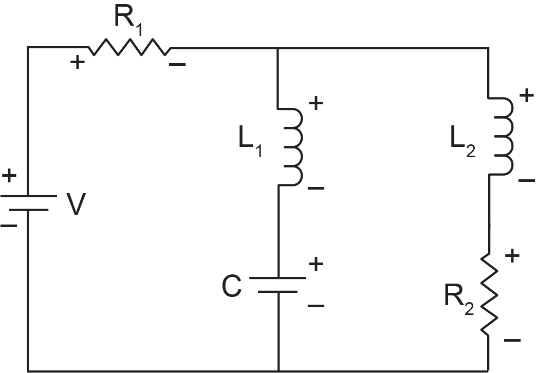
The following video shows how to build and run the model for this example in 20-sim.
The simplified BG model with a supplied voltage signal as a square wave is shown in Figure 7‑9.
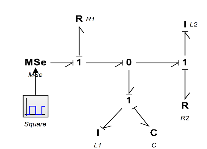
Figure 7‑10 shows an RCL three-loop circuit consisting of resistors, inductors, and a capacitor connected in parallel. We use the KCL approach to build the BG model for this example.
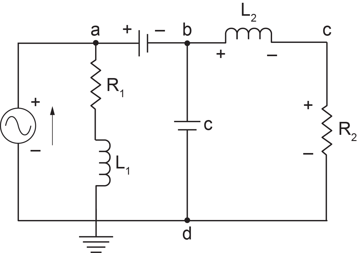
The following video shows how to build and run the model for this example in 20-sim.
The simplified BG model with a supplied voltage signal as a block wave is shown in Figure 7‑11.
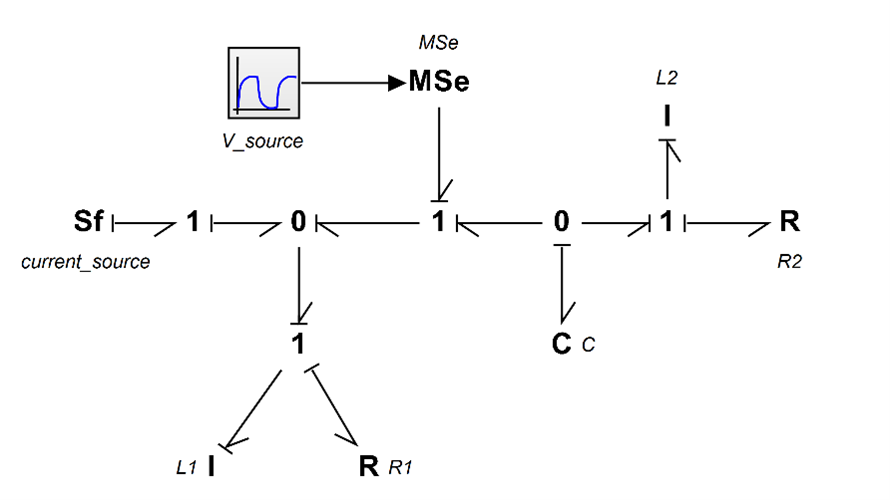
Figure 7‑12 shows a Wheatstone circuit consisting of resistors. This circuit is usually used to measure an unknown resistor, e.g., placed in the system as  , by adjusting the variable
  such that the current through
  is null, i.e., the balanced point. Using Kirchhoff’s and Ohm’s laws [25], we can calculate the currents going through the branch
  as
as  and branch
  as
as  Therefore, the voltages at nodes and , with reference to the ground, are
  and
and  , respectively. For having null voltage across , we let
  or after some manipulations, we get
  . As shown, the balanced point is independent of the voltage supplied. We use the KCL approach to build the BG model for this example.
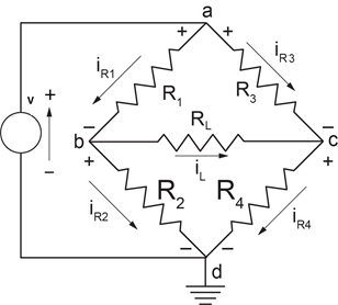
The following video shows how to build and run the model for this example in 20-sim.
The simplified BG model with a supplied voltage is shown in Figure 7‑13.
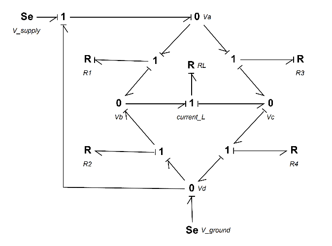
Figure 7‑14 shows an RCL multi-loop circuit consisting of resistors, inductors, and capacitors connected in series and parallel. We use the KCL/KVL approach to build the BG model for this example.
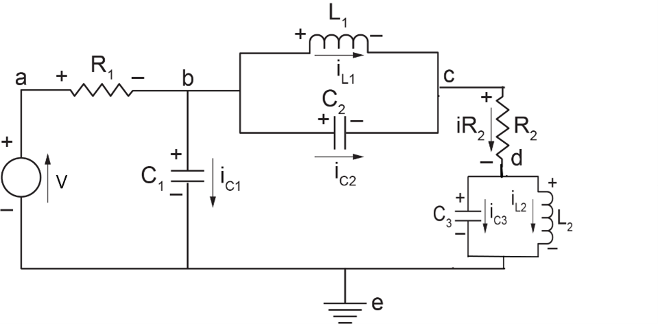
The following video shows how to build and run the model for this example in 20-sim.
The simplified BG model with a supplied voltage is shown in Figure 7‑15.
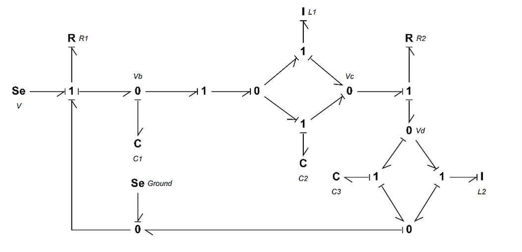
Figure 7‑16 shows an RCL multi-loop circuit consisting of resistors, inductors, capacitors, and a transformer connected in series and parallel. We use the KCL/KVL approach to build the BG model for this example.
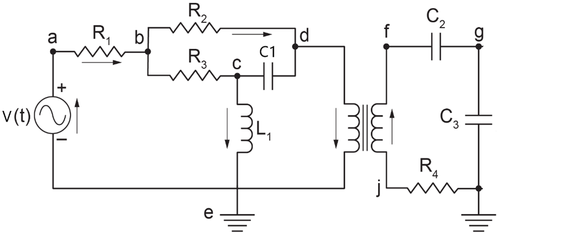
The following video shows how to build and run the model for this example in 20-sim.
The simplified BG model with a supplied voltage is shown in Figure 7‑17.
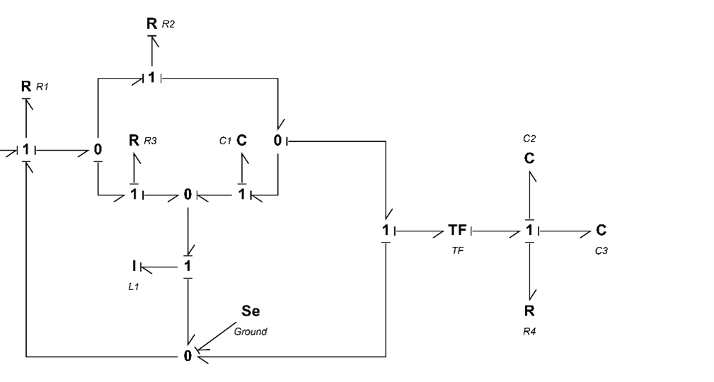
Exercises
Use following data:  ,
,  ,
,  ,
,  ,
,  ,
,  ,
,  , and transformer parameter 2:1. Perform Parameter Sweep on a range of parameter values, 0.5-3 and graph the results for electric charge on capacitor .
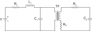
 ,
,  ,
,  for simulation. Report voltages across each element for a direct source voltage of
  . Also, run the model for a range of capacitance
  ,
,  ,
,  using Parameter Sweep and report the across the inductance for these values. Draw the sketch.
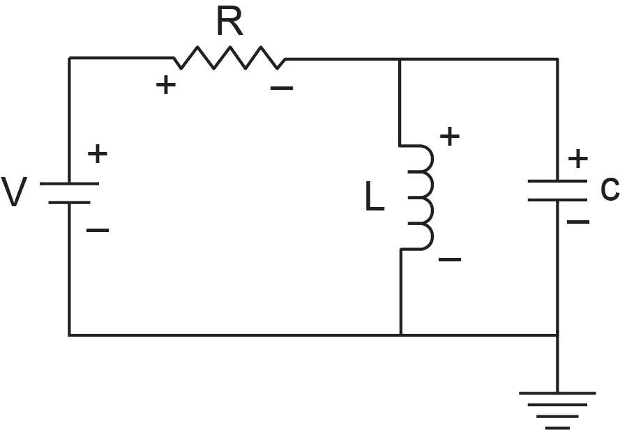

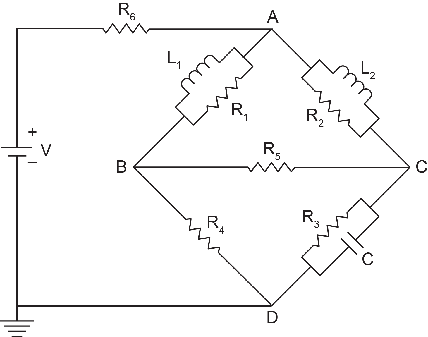
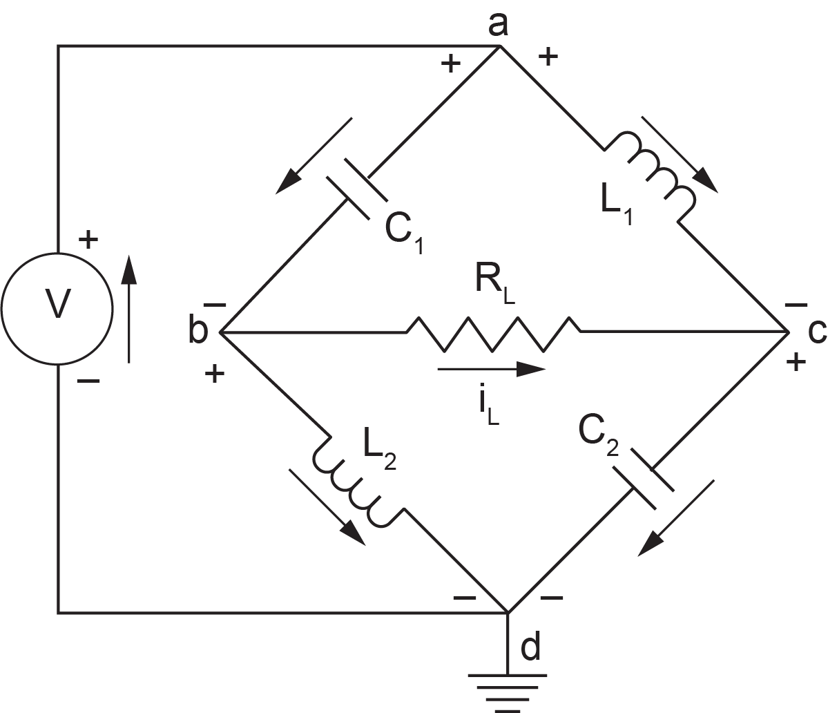
to be laid out in parallel. Build the BG model for the modified circuit. , , , , ,
  , ,
, ,  .
.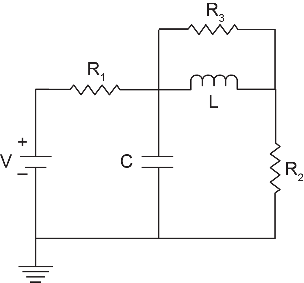
8
The generalized BG elements and relations apply to the modelling of dynamics of hydraulic systems in a similar way that the mechanical or electrical systems were treated; i.e.; they are analogous (see Table 3‑1). In this chapter, we define the effort and flow for hydraulic systems and derive the relations for hydraulic capacitance, inertance, and resistance corresponding to BG elements , , and , respectively. Note that the complexity of fluid behaviour in static or dynamic flow conditions require us to pay more attention to identify these quantities and relations as compared to those for mechanical and electrical systems.
For modelling hydraulic systems, we are usually interested in having a relationship between pressure and fluid volume in static conditions and between pressure drop and fluid volume flow rate in dynamic conditions. For example, we might be interested to know the pressure drop for a given flow rate in a pipe, or we might want to know the pressure at a given depth in a storage tank, as sketched in Figure 8‑1.
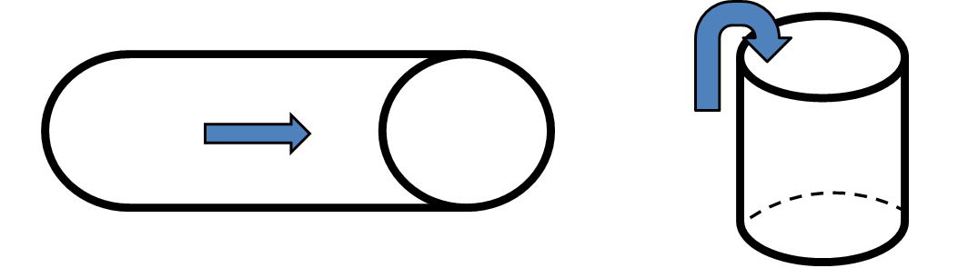
Recall that power is the quantity of interest in BG method (see section 3.2). Considering a control volume  of an incompressible fluid flowing under pressure
  , we can write the power as the product of the force exerting on the fluid, resulted from applied pressure, and the velocity of the fluid flowing through the volume, or
  But the velocity of the fluid can be written as
  , using the continuity relation, where
  is volume flow rate of the fluid and
  is the cross-sectional area of the control volume. Therefore, after substitution, we get
  , or equivalently rate of energy
  . Comparing the relation
  with the BG generalized relation for power, i.e.,
  , we can write
  and
and  . In other words, for hydraulic systems, pressure is equivalent to BG effort, and fluid volume flow rate is the BG flow. Similarly, we can write the generalized BG displacement as the volume of the fluid, or
  .
.
In BG method, the generalized momentum is the integral of effort. Therefore, we can write the fluid momentum  as the integral of pressure, or
  . Summarizing these relations, we have

Fluid compliance or hydraulic capacitance describes potential energy storage with a fluid, e.g., the height of fluid in a tank. It is equivalent to mechanical spring compliance or electrical capacitor capacitance. For a -element in BG method, we have . Using equivalent quantities for hydraulic systems, we can write  , or fluid compliance is volume change per unit of pressure acting on the fluid volume. For an incompressible fluid with density
  , the hydrostatic pressure at depth
  is
is  and the volume of the fluid is
  . After substitution, we get
  , or after rearranging and simplifying, the hydraulic capacitance for incompressible fluid is
(8.1) 
where is the gravitational acceleration. The dimension of fluid compliance can be worked out as ![[\dfrac{m^4s^2}{kg}]](https://pressbooks.bccampus.ca/engineeringsystems/wp-content/ql-cache/quicklatex.com-d754f821dd0f3326a4d2bd869614763b_l3.svg "Rendered by QuickLaTeX.com") = [
= [ ] =
] =  .
.
Note that the pressure could be replaced by total dynamic pressure for fluid in motion.
If the fluid is compressible, we use the bulk modulus of elasticity  for calculating the change in volume. By definition, is pressure needed to change fluid volume per unit of volume, or
  . Therefore,
  .
.
(8.2) 
For more complex flow and non-uniform, flexible tubes, consult with chapter 4 of Dean, Karnopp, Margolis, and Rosenberg [20].
Having the hydraulic capacitance, we can write the relation between the flow rate and the pressure as  , useful to calculate the flow rate for given pressure. Similarly, we can write
  , useful for calculating pressure for given flow rates.
(8.3) 
Note the similarity between relations given by Equation (8.3) and those given for mechanical spring (when pressure is replaced by force and fluid volume flow rate by velocity) and electrical capacitance (when pressure is replaced by voltage and fluid volume flow rate by current).
Fluid inertia, or hydraulic inertance, describes kinetic energy storage with a fluid or the inertia, e.g., of a fluid flowing in a pipe. It is equivalent to inertia related to mass in mechanical or inductance in electrical systems. For an -element in BG method,  describes the relation between generalized momentum and flow. Using equivalent quantities for hydraulic systems, we can write
  , or fluid pressure momentum is the product of fluid inertia by its volume flow rate. To derive the relation for , we require to have the relationship between the momentum and volume flow rate of the fluid flow. For derivation, we consider a control volume with length
  and cross-sectional area of the fluid with density , as shown in Figure 8-2.
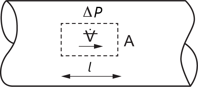
Assuming a pressure difference  between two ends of the control volume acting on the fluid, we can write Newton’s second law for the fluid motion as
 . Rearranging the terms and integrating the pressure, we get the pressure momentum
  . But volume is
  . After substituting, we get the relationship between pressure momentum and the volume flow rate as
(8.4) 
Comparing Equation (8.4) with the generalized momentum equation for -element, we can write the fluid inertia as
(8.5) 
The dimension of fluid inertia can be worked out as ![[\,\dfrac{kg}{m^4}]\, \equiv \dfrac{pressure\: momentum}{volume\: flow \:rate}](https://pressbooks.bccampus.ca/engineeringsystems/wp-content/ql-cache/quicklatex.com-d3751e078f0411692978b639f2e18e3c_l3.svg "Rendered by QuickLaTeX.com") .
.
From Equation (8.5), we can conclude that a fluid has larger inertia when flowing in small diameter tubes, compared to in larger tubes because is inversely proportional to . This effect is counterintuitive and is sometimes misinterpreted with the wrong assumption that large-size tubes should exhibit larger inertia effects. Note that we consider only force due to pressure, and not friction due to viscosity, assuming an ideal fluid.
For more complex flow and non-uniform and/or flexible tubes, consult with chapters 4 and 12 of Dean, Karnopp, Margolis, and Rosenberg [20]. For example, if the cross-section of the pipe and the density of fluid change along its -axis, then we get
(8.6) 
Having the hydraulic inertance, we can write the relation between the flow rate and the pressure as  , useful to calculate the flow rate for given pressure. Similarly, we can write
  , useful for calculating pressure for given flow rates.
(8.7) 
Note the similarity between relations given by Equation (8.7) and those given for mechanical systems (when pressure is replaced by force, fluid flow rate by velocity, and inertance by mass) and electrical systems (when pressure is replaced by voltage, fluid flow rate by current, and inertance by inductance).
Fluid, or hydraulic, resistance describes energy dissipation with a fluid, e.g., friction of a fluid flowing in a pipe. Fluid resistance is equivalent to dampers in mechanical or resistors in electrical systems. For an -element in BG method, we have  Using equivalent quantities for hydraulic systems, we can write
(8.8) 
or fluid resistance is equal to pressure change per unit volume flow rate. This relationship depends on the state of the flow (e.g., laminar, turbulent) and the fluid properties (e.g., ideal, viscous,) [26], [27], [28]. Note the similarity between relations given by Equation (8.8) and those given for mechanical systems (when pressure is replaced by force and fluid flow rate by velocity) and electrical systems (when pressure is replaced by voltage and fluid flow rate by current).
To demonstrate the derivation of the relation for , we consider a laminar flow of a viscous incompressible fluid in a pipe (so-called Hagen-Poiseuille flow) and write Newton’s second law for a cylindrical differential control volume of the fluid with length  along the pipe axis and a cross-section with radius , as shown in Figure 8‑3. This flow is axisymmetric, and the velocity profile changes along the radius related to a cylindrical coordinate system
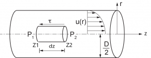
For a steady flow (i.e., non-transient), we have 
 . But the forces applied on the fluid are due to pressures
  at point
  and
and  at point
  and the viscous-induced shear stress
  . Hence,
  where is the radial dimension in the plane parallel to the pipe cross-section. We need the relation for fluid friction effect due to viscosity. According to Newton’s law for a viscous fluid, we have
  , assuming the shear stress due to the fluid’s viscosity be proportional to the velocity gradient along the radius with the proportionality constant being the dynamic viscosity
  . Note that velocity profile at any cross-section of the pipe is only a function of radius, or velocity vector is
  . After substitution, we have
  . After simplifying and rearranging the terms, we have
  . Integrating the latter relation, noting that velocity is not a function of , gives
  , or
, or  . Now, we rearrange the terms and let
  , the length of the control volume, and use the pressure difference as a positive constant quantity
  in the direction of the fluid flow. Hence,
  . Integrating both sides (the left-hand side with respect to
  and the right-hand side with respect to ) gives
  . The constant of integration can be obtained using the information at the boundary of the pipe assuming the no-slip condition, or
  , where D is the pipe diameter. Therefore,
  . Hence, after back substitution, we get the velocity profile
  . This relation is the famous parabolic velocity profile for the flow in a pipe and can be written in its functional form as
(8.9) 
Using Equation (8.9), we can calculate the velocity for any given value of , e.g.,  at the centre-line of the pipe or at the interior wall of the pipe.
Now, to find the volume flow rate, we integrate the velocity  over the whole cross-section of the pipe using a differential area element
  . Or, the volume of the fluid passing through the whole cross-section of the pipe per unit of time is given by
 , or
, or
(8.10) 
Comparing Equation (8.10) with Equation (8.8), we can write the fluid resistance as
(8.11) 
The fluid resistance can be interpreted as the amount of pressure drop per unit of volume flow rate of the fluid in the pipe. The dimension of fluid resistance can be worked out as ![\Big[\dfrac{kg}{s.m^4}\Big] = \Big[\dfrac{N.s}{m^5}\Big]\equiv \dfrac{pressure}{volume\: flow\: rate}](https://pressbooks.bccampus.ca/engineeringsystems/wp-content/ql-cache/quicklatex.com-2fb967c37fd0bbdb012a7b092c07051a_l3.svg "Rendered by QuickLaTeX.com") .
.
Other BG elements for hydraulic systems are sources of flow (e.g., centrifugal pumps) and efforts (e.g., reservoirs, tanks, displacement pumps). Pumps provide flow of a fluid at a certain flow rate according to their types and specifications. Reservoirs or pressure chambers provide certain pressure to the system as an effort source. The transformers elements are those like piston-cylinder (plunger), and gyrators are those elements like reaction turbines or hydraulic motors. Sketches below show some related elements.
Typical hydraulic components are shown in Table 8‑1.
| -element (valve) | -element (storage) | -element (fluid mass) | -element (plunger) | -element (pump) |
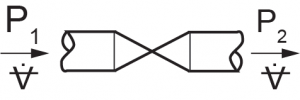 | 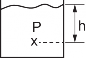 |  | 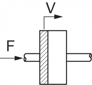 | 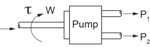 |
The sign convention for hydraulic systems can be defined by specifying the relative high/low pressure points in the system and, hence, the positive fluid flow direction along the pressure drop. The pressure reference is commonly taken to be the atmospheric pressure (i.e., one atm for absolute and zero for gauge pressures). For BG modelling, it is recommended to have all pressures in gauge and define a zero-pressure point for reference atmospheric pressure. If the results are required in absolute pressure units, then one unit of atmospheric pressure can be added to the obtained values from the BG model.
As mentioned in chapter 4, the general guidelines for drawing BG models can be applied to hydraulic systems, along with causality assignment rules. For hydraulic systems, we follow the guidelines given for electrical systems (see section 7.3) as described in the following steps:
1) Assign sign convention for fluid flow directions.
2) Assign 0-junction for each distinct pressure point in the system.
3) Assign 1-junction for each element in the system. This is for taking care of relative pressure drops related to each element located between two adjacent 0-junctions, since 1-junction is effort summator.
4) Select a node in the system as a reference, i.e., the atmospheric pressure point, and assign a 0-junction element to it. If gauge pressures are used, then this 0-junction and all connected power bonds can be eliminated to simplify the model.
5) Assign -element for storage/capacitors, -element for friction, -element for fluid mass, and for pressure and for flow sources.
6) Assign -element for hydraulic transformers and -element for hydraulic gyrators.
7) Connect the elements with power bonds and assign causalities. Simplify by neglecting the bonds and the 0-junction which are connected to the 0-junction representing the atmospheric pressure.
Similarly, a 1-junction-based approach can be used for distinct flow rates and hence simplifying the BG model, as we demonstrated in the previous chapter with electrical systems.
Figure 8‑4 shows a hydraulic system consisting of two tanks, pipes, and valves. Build a BG model for this system.
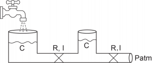
Solution:
We follow the systematic procedure for building the BG model, listed in section 8.7. For this system, we can easily identify two pressure points located at the bottom of tanks. We assign two 0-junctions for each. For flow input, we assign a flow source element, and for the output, an effort source element to define the atmospheric pressure at that location. For the tanks, we only consider capacitance, assuming slow fluid motion and neglect inertia and friction (i.e., no inertance nor resistance). For the pipe sections, we consider inertance and resistance. As well, we assign 1-junctions for flows in the pipes that represent the pressure changes for these components. Figure 8-5 shows the resulting BG model.

In this example, we use the BG model developed in section 8.8, along with data assigned to parameters for simulation. Considering water as the fluid ( ) and the data given in Table 8‑2, we can calculate the related , , and of the elements in the system. The diameter of the pipes is 15 cm, and
  .
.
The following video shows how to build and run the model for this example in 20-sim.
| Component |  -section area -section area[  ] ] | Length [ ] | [  ] ]Eq. (8.1) | [  ] ]Eq. (8.5) | [  ] ]Eq. (8.11) |
| Storage tanks | 2 | – |  | – | – |
| Pipe1 | 0.01767 | 4 | – | 226372.4 | 322 |
| Pipe2 | 0.01767 | 2 | – | 113186.2 | 161 |
In this example, we use the BG model developed in section 8.8, adding a pump to the system as shown in Figure 8‑6. In this example we discuss in more detail the BG model of a pump. For further details related to BG modelling of pumps, consult with references cited as [21] and [29].
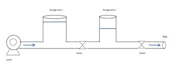
The following video shows how to build and run the model for this example in 20-sim. The resulting BG model is shown in Figure 8‑7.
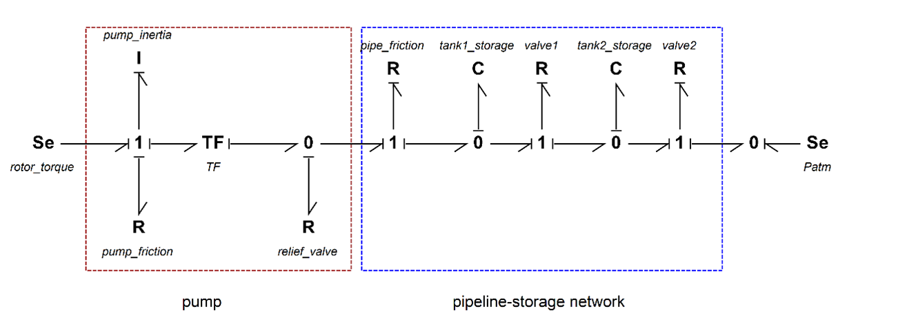
In this example, we consider a hydraulic lift, as sketched in Figure 8‑8. We build a BG model for this hydraulic system. The continuity relation applies to the fluid motion and Pascal’s law defines the pressure distribution of the fluid in the cylinders. Two transformer elements are used in the BG model to convert linear velocities of the pistons to/from volume flow rate and convert forces to pressures (see Figure 8‑9). The transformers’ parameters are explained in the video clip.
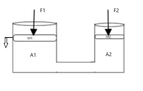
The following video shows how to build and run the model for this example in 20-sim.
The BG model is shown in Figure 8‑9, along with the detail of the transformers’ inputs and outputs.
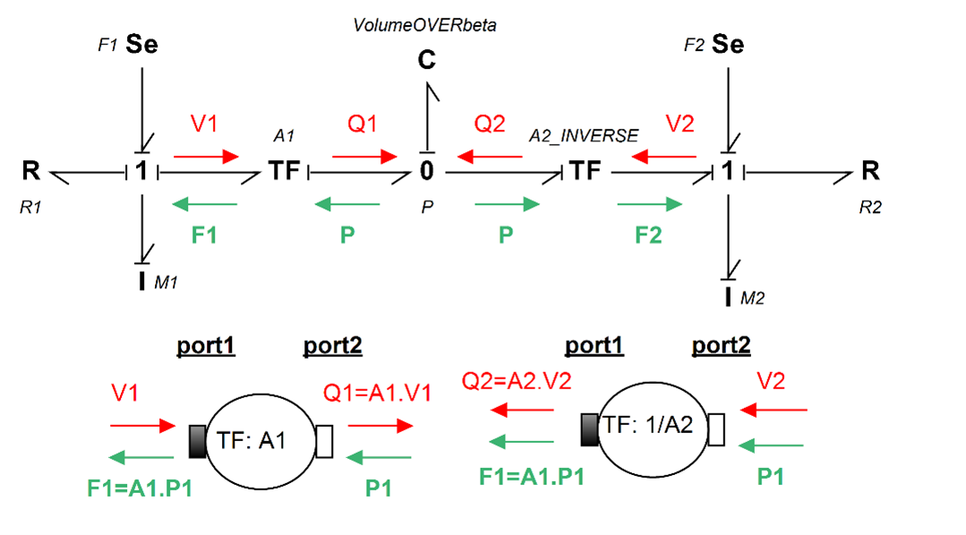
Exercises
9
As mentioned in previous sections (see chapter 3), the universality of BG elements for application to analogous quantities is the main strength of this method for modelling and simulation of multi-domain systems. In practice, many systems are composed of multi-energy domains, e.g., an electric motor turning a mechanical shaft, a car engine generating and transferring power to the torsion shaft, a wind turbine, a robot. The BG modelling method can serve as a powerful tool for modelling these real-world systems.
In this chapter, we present several examples of multi-domain systems and build their BG models. We emphasize that the control sub-system is a major part of any engineering system. In this textbook, however, we focus on BG method and how to build BG models for systems. The full treatment of the topic of control is left for a possible future volume. For information about control theory and modelling, consult with references such as those cited as [20], [21], [30], and [31].
For this example we consider a car brake system as shown in Figure 9‑1. The driver applies a force on the brake pedal, which is transferred to the brake discs through the hydro-mechanical system. The process of force transfer is modelled with using several transformer elements ().
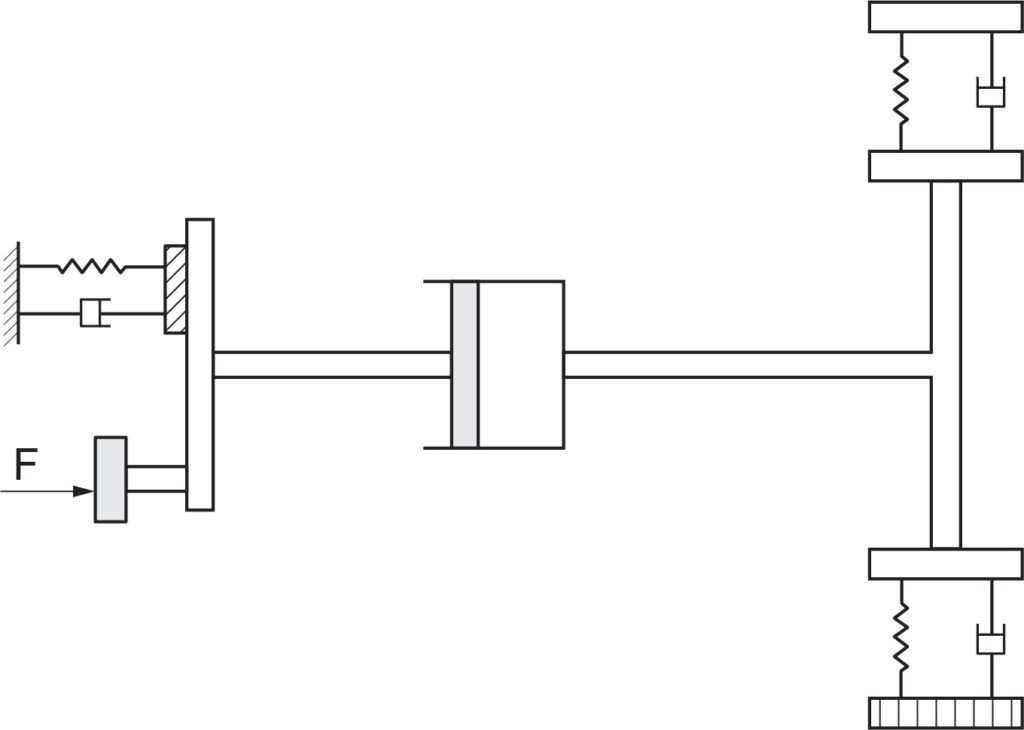
The following video shows how to build and run the model for this example in 20-sim.
The BG model for this system is shown in Figure 9‑2. For further reading, consult with the reference cited as [32].
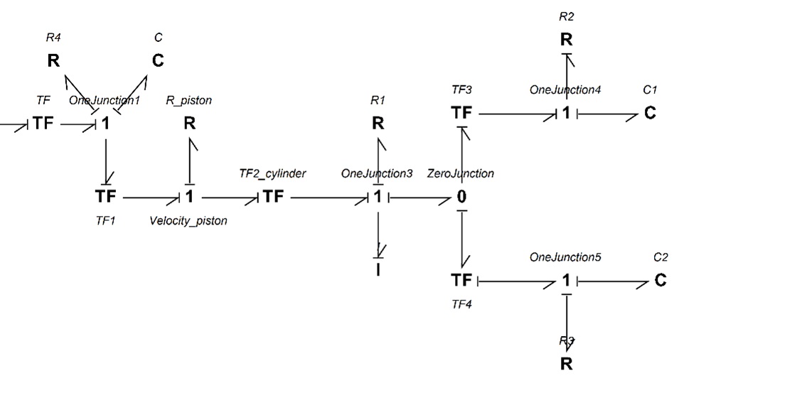
For this example, we consider an electro-mechanical hoist system as shown in Figure 9‑3. The electric motor is connected to a shaft-drum mechanical system. The load is represented by a mass connected by an elastic extensible string to the hoist drum. A gyrator () and a transformer () elements are used in this model. The -element models the electric motor by transforming the motor voltage (current) to the angular velocity (torque) of the drum/shaft and the -element transforms the angular velocity of the drum to the linear velocity of the mass.
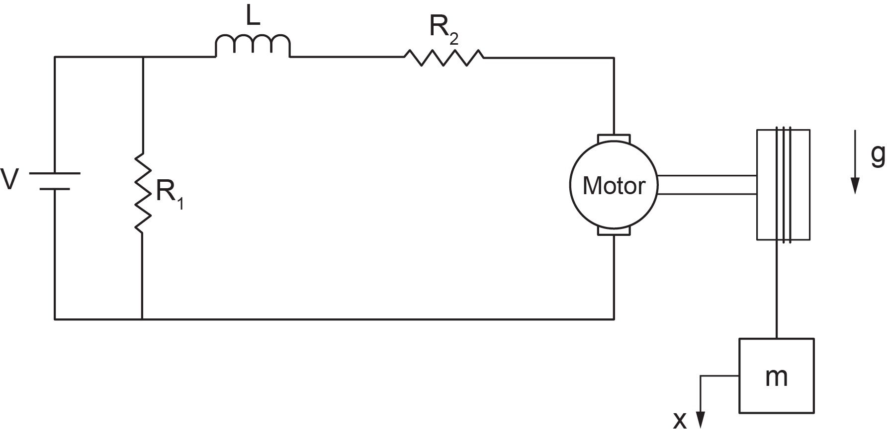
The following video shows how to build and run the model for this example in 20-sim.
Figure 9‑4 shows the BG model for this system. For further reading, consult with the references cited as [21] and [33].
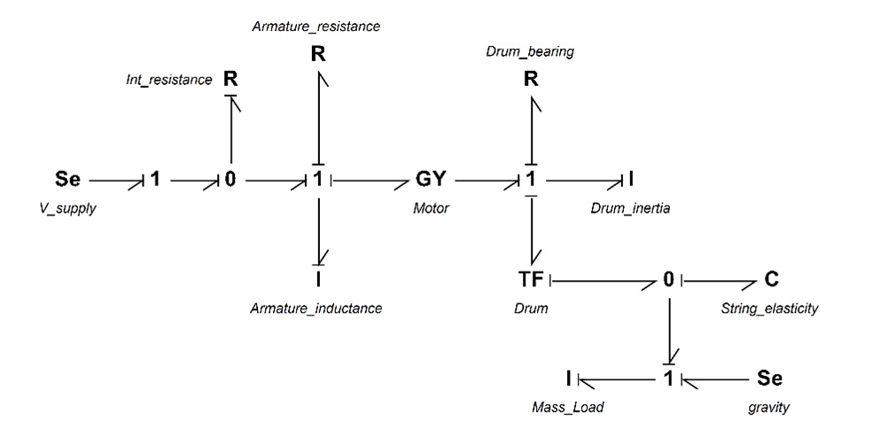
For this example, we consider a mechanical drive shaft system carrying a torsional load as shown in Figure 9‑5. The applied torque is transferred to the gear-shaft system. The load can be applied through an electric motor (not shown). This model uses several transformer elements (). The -elements exchange the angular velocity of the gears, using compatibility requirement.
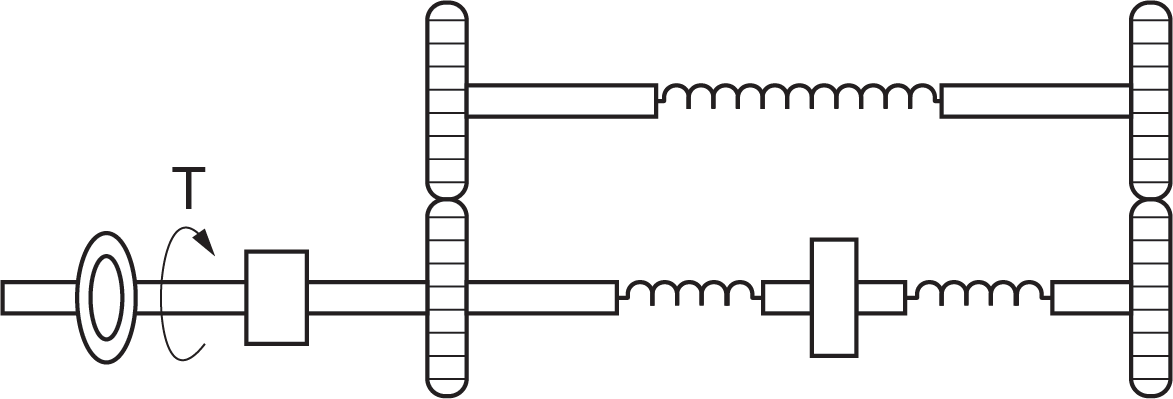
The following video shows how to build and run the model for this example in 20-sim.
The BG model for this system is shown in Figure 9‑6. For further reading, consult with the references cited as [20] and [34].
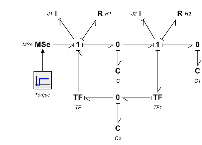
For this example, we consider an inverted double pendulum system pivoted to a moving mass, as shown in Figure 9‑7. The rods are pinned together, and each has one rotational DOF, represented by  and
and  . The centre of mass is located at the mid-points
  and
and  of each rod, represented by
  and
and  ; associated mass by and ; and rotational moment of inertia by
  and
and  . The motion is measured with reference to a fixed coordinate system, , initially at origin. Applied force is exerted on mass , moving horizontally with its displacement designated by .
The coordinates of the centre of mass for the rods are given as  ,
,  , and
, and  ,
,  . Therefore, the corresponding velocities are
  ,
,  ,
,  , and
, and  . Assuming small angles, or
  and
and  , we get
  and
and

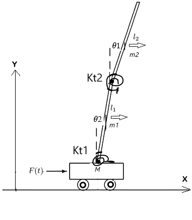
The following video shows how to build and run the model for this example in 20-sim.
Figure 9‑8 shows the BG model for this system. For further reading, consult with the references cited as [20] and [32].
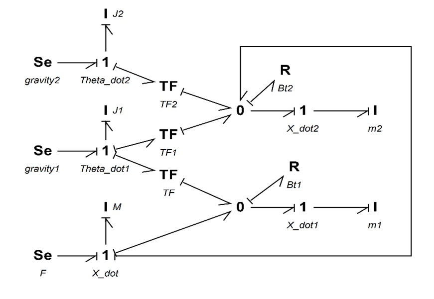
Exercises
10
Studying the behaviour of systems with respect to time is the primary approach for systems modelling and analysis. However, when a system behaves in a repetitive mode under some applied load and/or boundary conditions—a quasi-static mode—we are interested in the changes in terms of the inherently-involved frequencies of the system rather than the details of instantaneous variations with respect to time. Therefore, transforming the domain of analysis from time to frequency provides us with useful and important information about the behaviour of systems. For example, identifying characteristics of a system—such as its natural frequency, behaviour at large and small frequencies, and magnitude of certain quantities at specific frequencies—provides useful insights in terms of system analysis, design, and control.
In this section, we present a brief background of frequency analysis and methods with focus on Bode plot method and transfer function, with worked-out examples. However, this textbook does not present a full discussion of control theory and related methods for system analysis.
For further reading, consult with references cited in this chapter. 20-sim has tools for performing frequency analysis using BG models and for drawing Bode plots for systems. Through some examples, we will demonstrate how to use these tools.
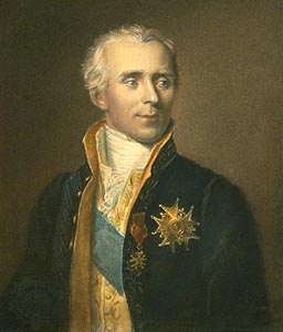
Performing analysis in frequency domain requires a transformation from time domain to frequency domain. Having a mathematical model describing the behaviour of a system, we can use a transformer to convert the governing equations from time domain to frequency domain . Using applied engineering mathematics, we usually employ Laplace and/or Fourier transforms for such an operation. The Laplace transform (defined in complex  -domain) is a more general case of Fourier’s transform (defined in -domain), as given below for transforming a function of time , [12], [35].
(10.1) 
where  and for
  these two transforms are comparable. Note that, in principle,
  but the real part,
  of complex variable , is not included here since we are interested in equilibrium at a steady state in frequency analysis. Application of these transforms greatly simplifies the solutions of system equations, both for ODEs and PDEs. The original functions in time domain can be calculated back using the inverse transforms of Laplace and Fourier, given as
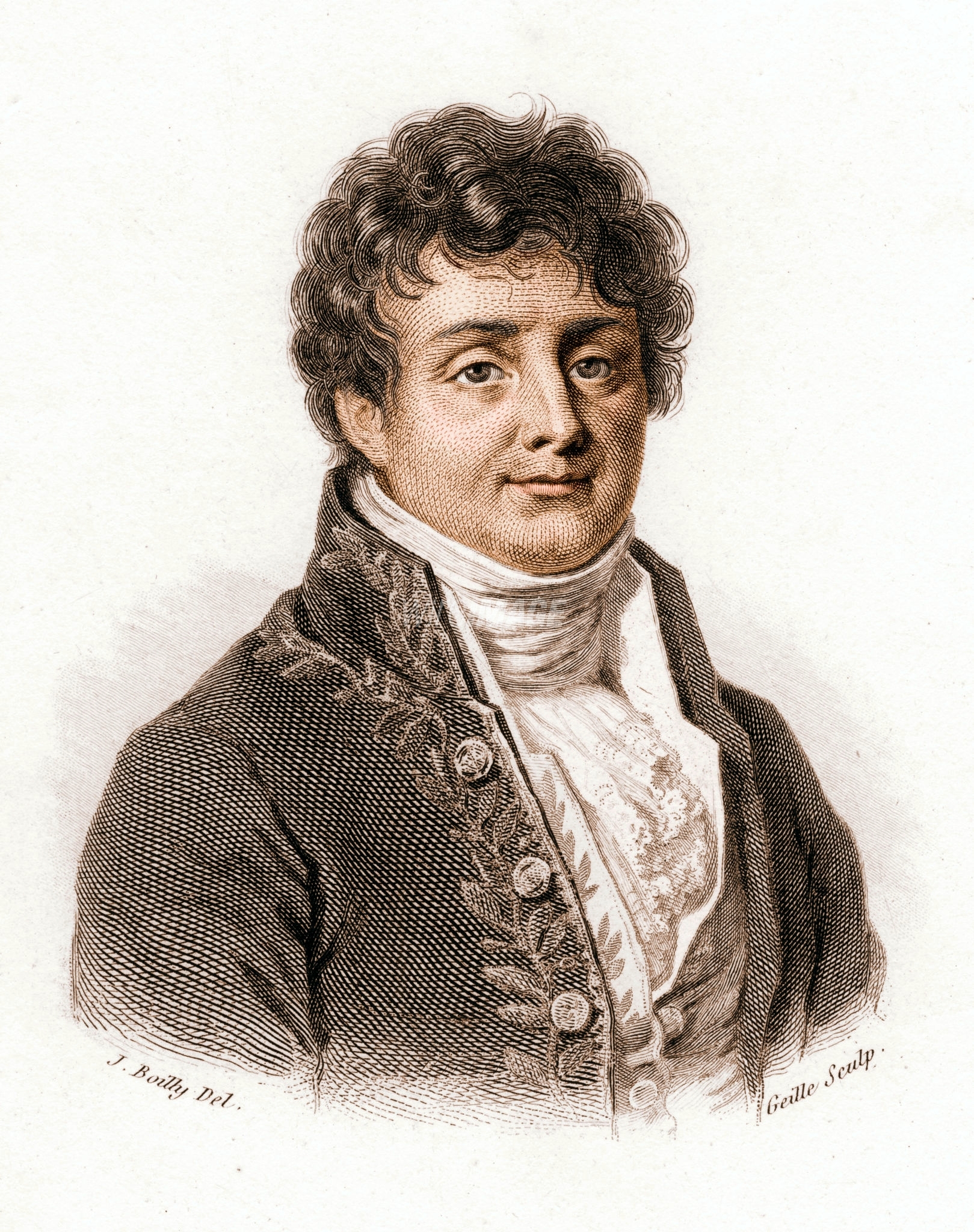
(10.2) 
In control theory for systems, several methods are used for studying system behaviour and design, including Bode and Nichols plots requiring frequency-domain response representation, root-locus method requiring complex-domain pole-zero representation, and polynomial-domain design requiring transfer-function representation [31], [36]. A transfer function, by definition, is the ratio of the output signal (i.e., magnitude, power) of a system over selected input signal values. Among these methods, we focus on Bode plots for application in system design using BG models. Bode plots are used for linear systems or linearized non-linear systems. For more detail, see Reference Manual 20-sim 4.6. To access the manual, from the 20-sim Editor window, go to Help, and then select Manual (PDF).
A linear system, or LTI (linear time invariant), is a system for which the linear combination of output of a set of inputs is equal to the sum of outputs resulting from each input, e.g., as shown in Figure 10‑1.
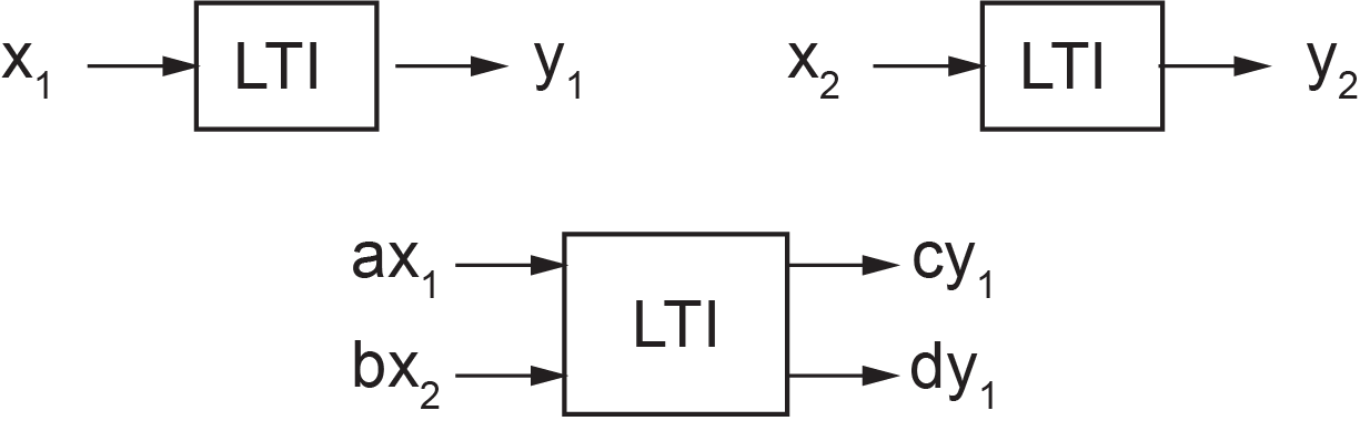
Considering a proportional integral (PI) controller (for which the output is equal to the input multiplied by a constant and added to the integral of the input), we provide a sinusoidal signal input with frequency of 0.5 rad/s (or  ) given as 0.5. Assuming the constant multiplier to be 2, we get the output as
  ). From the output, we observe that the frequency remains the same as that of the input. Now, by multiplying
  to the output, we rewrite it as a single sinusoidal function, or:

Therefore, the input amplitude is magnified by a factor of  , frequency remains the same as mentioned, and a phase change of
  is introduced to the output signal by the PI controller. But one can ask the question: what would be the controller response to a similar signal with a different frequency? For example, if we repeat the same calculation for an input signal given as
  , we get the response
  . To find the response to a spectrum of input frequencies, in principle we can repeat similar calculations and analyze the system behaviour. Table 10‑1 shows some typical response result for input signals of the form
  into a PI controller.
| Frequency (rad/s), | Response Amplitude | Response Phase (deg.) |
| 0.1 | 10.198 | -78.690 |
| 0.2 | 5.385 | -68.199 |
| 0.3 | 3.887 | -59.036 |
| 0.4 | 3.202 | -51.340 |
| 0.5 | 2.828 | -45.000 |
| 0.6 | 2.603 | -39.806 |
| 0.7 | 2.458 | -35.538 |
| 0.8 | 2.358 | -32.005 |
| 0.9 | 2.288 | -29.055 |
| 1 | 2.236 | -26.565 |
| 2 | 2.062 | -14.036 |
| 3 | 2.028 | -9.462 |
| 4 | 2.016 | -7.125 |
| 5 | 2.010 | -5.711 |
| 6 | 2.007 | -4.764 |
| 7 | 2.005 | -4.086 |
| 8 | 2.004 | -3.576 |
| 9 | 2.003 | -3.180 |
| 10 | 2.002 | -2.862 |
One can make graphs of the response amplitude and phase changes versus input frequency to study the behaviour of the PI controller used in this example.
The results of the calculations mentioned in section 10.3 motivate us to look for a more general and practical method of frequency analysis of systems. The calculations presented are laborious, although new computer tools, e.g., Excel or even computer coding can speed up the process. However, Hendrik Wade Bode, working at Bell Labs in the 1930s, suggested a more practical and now commonly used graphical method—Bode plots, [21], [31], [37], [38]. This method has a wide range of applications in system dynamics, control, and design. An important outcome of having Bode plots for a system is a quick visual insight into the system’s dynamical behaviour for a wide range of frequencies.
In this section, we present the basic idea and some formulas related to Bode plots and what they intend to represent when applied to a system.
Following the example presented in section 10.3, we assume, without losing generality, to have an input sinusoidal signal to the PI controller with frequency given as  . The output is, then,
  with amplitude
  and phase
  . The relations for the output amplitude and phase angle depend on the PI controller specifications. For our example having a proportionality factor of two and an integration, using similar manipulations as those given in section 10.3, we find
  and
and  . Now, after transforming the input and output signals to the Laplace -domain, using Laplace transform (see Equation (10.1)), we get
  and
and  . The transfer function
  (also referred to as gain function) is defined as the ratio of the output amplitude over input amplitude. For our examples, we get, after some simplifications,
  . Having the transfer function, we can substitute , to transform from -domain to -domain, guided by Equation (10.1). Therefore,
  , or the transfer function in frequency domain. This is a function of a complex variable and can be written, in general, as its real and imaginary parts or
  . Therefore, after some manipulations, we get
  . This gives the real part
  and imaginary part
  . Therefore, the magnitude of the transfer function is
  . The relations for transfer function including its magnitude and phase are summarized in Equation (10.3).
(10.3) 
A set of plots consisting of magnitude  and versus logarithm (at base 10) of is called Bode plots. However, magnitude is traditionally measured in decibel (dB), phase angle in degrees, and frequency as logarithm of frequency in rad/s (or in Hz).
Recall that dB (one tenth of a bel) is a unit for measuring the power of a signal with reference to a threshold. For example, the threshold for human hearing is  , given as power intensity; dB is measured in logarithm of the power ratios at base ten, or
  . But since power of a wave signal is proportional to its amplitude squared, then we get
  , or
, or
(10.4) 
Therefore, Bode plots are composed of two charts: signal gain in dB and phase in degrees versus logarithm of , usually given in a single graph chart. The graphs in Figure 10‑4 show the Bode plots for the PI controller, generated using 20-sim. The tools available for drawing Bode plots in 20-sim can also be used when a transfer function is available or calculated and also after a BG model is built for systems. For this example, we calculated the transfer function and used it to draw the corresponding Bode plots. For drawing the corresponding Bode plots, follow these steps:
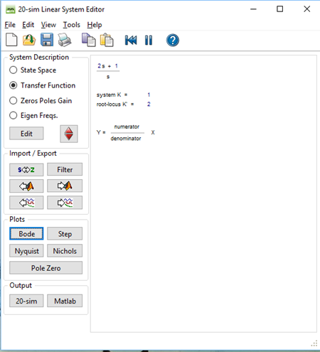 . For this example, having
  the coefficients for the numerator polynomial are (2, 1) and for the denominator polynomial are (1, 0). Note the zero term, i.e., the coefficient for the term
  , or the constant term. A space can be used instead of a comma, to separate the coefficients.
 at low frequencies to null at high frequencies. Therefore, the PI controller is in phase with the input signals at high frequencies and out of phase, by about , at low frequencies.
 (also referred to as corner or break frequency). This frequency is defined when the output power reaches to 50% of the input signal power (so-called half-power point), or
  .
. ) is at about 6.02 dB. Hence, the cutoff frequency corresponds to the point at 6.02+3=9.02 dB, or
  using Equation (10.4). This gives the cutoff frequency of
  rad/s, using
  . At the cutoff frequency the phase reads
  deg, using
  , after conversion.
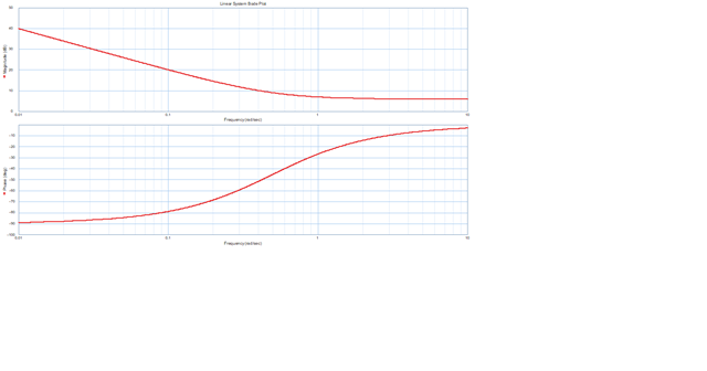
By following the steps presented in the following section, we can also draw Bode plots using 20-sim when a BG model of a system is available.
After using 20-sim to build a BG model, to draw related Bode plots, click on Tools and select the options in the Frequency Domain Toolbox to draw related Bode plots. We can draw Bode plots using transfer function, either manually or using computer graphing tools. The following steps can be used for drawing Bode plots, by either (A) using 20-sim software tool or (B) manually:
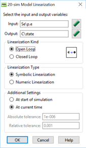
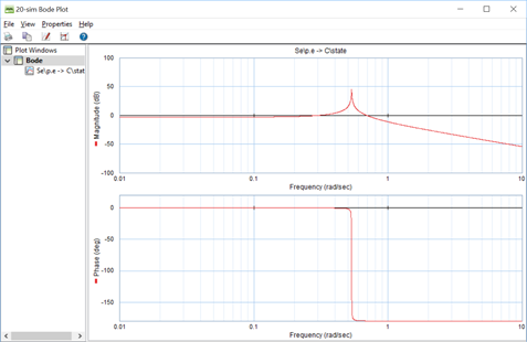 -domain, , using Laplace transform. into transfer function, to get
  ..
.. and power, using Equation (10.4).
Alternatively, Bode plots can be drawn using 20-sim after having the desired transfer function from step 1 above, by following the guideline given in section 10.4.
A system’s transfer function  is given. Find expressions for magnitude and phase angle and draw the corresponding Bode plots. Consider the frequency range 0.01–1000 rad/s. Discuss the system dynamical behaviour at low and high frequencies, including cutoff frequency.
Solution:
Using the guidelines, we substitute in . Therefore,  After multiplying and dividing by the conjugate of the denominator, we get
  . From this expression, we get the real and imaginary parts as
  and
and  . Using the real and imaginary parts and Equation (10.3), we can calculate the magnitude and phase as
  and
and  . Note that at
  and at
  . We can draw the Bode plots, manually or using 20-sim, for example. The cutoff frequency can be calculated as follows. The gain magnitude at
  reads
reads  . Therefore, the corresponding power is
  . The cutoff frequency corresponds to
  . Therefore, the corresponding gain is
  , using
  . After substituting for
  and using
  , we get cutoff frequency
  . The phase at the cutoff frequency can be calculated using
  or
or  .
.
Following the steps given in section 10.4, we can use 20-sim and the transfer function  to draw the Bode plots. The coefficients for the polynomials are (1) for numerator, and (1, 6, 8) for denominator. The resulting Bode plots are shown in Figure 10‑7.
The following video shows how to build and run the model for this example in 20-sim.
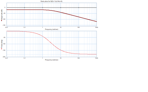
Build the BG model and its Bode plots considering transfer function based on force as input and displacement of the spring  as output. Use the mechanical system as shown in Figure 10‑8 with
 ,
,  ,
,  ,
,  ,
,  ,
,  ,
, 
 , and
, and  .
.
The damper  connects mass
  and the wall at the right side. Repeat the simulation for the following cases:
 to study its effect on the system with Parameter Sweep tool in 20-sim (available at the 20-sim Simulator window: select Tools > Time Domain Toolbox >Parameter Sweep). During the sweep, monitor the displacement of mass ., start time 2 sec, and stop time 3.5 sec.
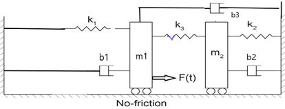
Solution:
The following video shows how to build and run the model for this example in 20-sim.
Figure 10‑9 shows the resulting Bode plots. Note that in this video, the force is applied to mass  , in the first try and then moved to mass according to the sketch shown in Figure 10‑8.
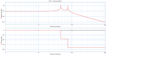
11
This chapter discusses several topics pertinent to modelling and simulation of systems dynamics with focus on BG method. The reader can consult with these sections as independent topics or as supplementary to previously discussed topics.
The product of conjugate variables related to a physical quantity should, by definition, give the corresponding quantity. In chapter 3, sections 3.2 and 3.5, we discussed the power variables (effort and flow ) and their relations to the state variables (momentum and displacement ). The product ( ) is power—so-called power variables—and integrating them, with respect to time, gives and , respectively. Hence the and are called energy variables. However, further attention to the dimension of the product of the variables, i.e., (
 ), indicates that the dimension of this quantity is not equivalent to that of energy. For example, in the SI system of units, we get
 ![[p.q] = [N.s.m] = [J.s]](https://pressbooks.bccampus.ca/engineeringsystems/wp-content/ql-cache/quicklatex.com-28113a3d6063e40d39bf86db53e483ce_l3.svg "Rendered by QuickLaTeX.com") . Therefore, we can call and conjugate power variables because the product () is power. But this definition does not apply to the product (). Instead, the product (
. Therefore, we can call and conjugate power variables because the product () is power. But this definition does not apply to the product (). Instead, the product ( ) or product (
 ) can be defined as true conjugate energy variables.
One can ask the question, what is the relationship among these variables? To investigate further and provide a possible answer, we consider the system energy function  . This functional form is legitimate, since we know that the energy stored, in storage elements and , is uniquely defined by state variables (see section 3.5). The total differential change of energy is then
  . In principle,
  . But the partial derivative
  can be ignored at equilibrium state of the system, or when and are kept constant and energy is not changing with time. Now, the total differential change of power
  can be written as the time derivative of energy, or
  . But
. But  and
and  , the effort and flow in BG method, respectively. Therefore, we can write
(11.1) 
Equation (11.1) clearly defines the relationship among power variables (effort and flow ) and state variables (momentum and displacement ) with respect to the power () and energy () of the system. Note that for a system, we can write this equation for each component and sum it up to get the relation for the system.
From Equation (11.1), we can conclude that by dimensional analysis,  has the dimension of flow and
  the dimension of effort, according to BG terminology. We define these quantities as system flow and effort, or (note that the partial derivative definition is explicitly shown here)
(11.2) 
For example, considering a mass, represented by an -element, its kinetic energy can be written as  , but
, but  , the velocity of the mass or the flow associated with the -element. Similarly, considering a mechanical spring with stiffness , represented by a -element, its potential energy can be written as
  , but
, but  , the force acting on the spring or the effort associated with the -element. Equation (11.2) applies analogously to mechanical, electrical, hydraulic, or thermal systems. Note that the energy function relates to the Hamiltonian of the system, [13].
Forces due to gravitational acceleration can be implemented in a BG model using effort source element . But it feeds power to the system when the assigned positive direction of displacement/velocity and the gravitational acceleration vector are in the same direction. Otherwise, the system feeds power into the gravity field, or loses power. In manually drawn BG, the direction of the power bond is drawn from toward the system when the gravity and displacement directions are matched; otherwise, the power bond should be toward the element. In 20-sim, however, it is not possible to draw a power bond pointing toward an element because it is defined as a source element. Hence, a negative value of is assigned to the associated parameter in the corresponding equation model, i.e., −9.81  (see Figure 11-1). Note that is interpreted as gravitational force per unit mass, here.
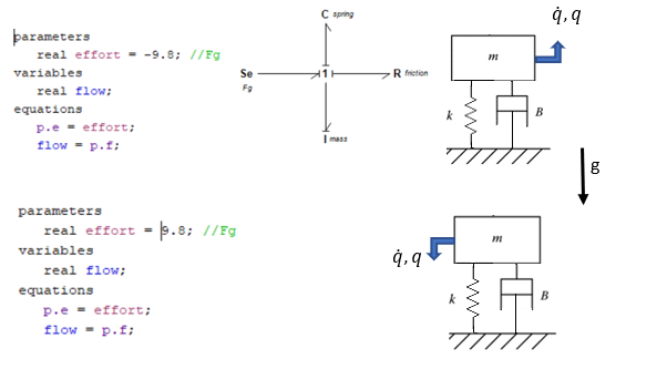
Although graphics of BG models can give us some insights into the dynamics of systems before actually solving the systems equations, having the mathematical model consisting of a system of equations is the ultimate goal resulting from a BG model, or for that matter, any model. In the previous sections, we discussed that for a BG model with integral causalities, we can derive a system of ODEs in terms of state variables, i.e., and (see section 3.5). For such a system, the number of equations, is equal to the sum of number of associated with – elements and number of associated with the – elements. In other words, the system equations are coupled first-order ODEs explicitly given in terms of state variables and can be solved simultaneously using numerical schemes. The solution of these coupled equations is, obviously, easier to obtain for linear systems rather than it is for non-linear systems.
In this section we discuss the procedure and guidelines of how to extract system equations from a BG model. For now, we assume that all storage elements (i.e., – and – elements) in the system are assigned with integral causality strokes. In the next section, we discuss cases when derivative causality and/or algebraic-loop situations may exist in a BG model, along with the definitions and resulting consequences for such systems equations.
Referring to the energy management of a system, we have already discussed that the energy input to a system is partially stored in storages and the rest is dissipated through dissipaters. Therefore, the storage elements are key elements for studying the dynamics of any system. This principle also applies to the BG models, and we use it to extract system equations.
The system equations can be given in a general form as  where , the vector representing time derivative of state variables,
  , the vector representing the inputs, with indices
  and
and  . One can expand this functional to get
(11.3) 
After building the BG model for a system, we ask the following two key questions, [21]:
Q1: What does each component/element send to the system?
Q2: What does the system send back to the storage components/elements?
Each question guides us to list the corresponding relations involving the state variables and performing some manipulations to write the system equations in terms of the state variables, using the general guideline of on and on . The following steps can be used to extract the system equations:
’s on ’s and all ’s on ’s, or momenta (or their derivatives) associated with the inertia elements and displacements (or their derivatives) associated with the capacity elements.Now, we present some worked-out examples to demonstrate the application of the above mentioned procedure.
For this example, we consider a mechanical system as shown in Figure 11-2. This systems has three DOF associated with three masses. The number of state variables is seven, associated with the storage elements, three masses, and four springs. The positive displacements are considered as shown, and tension forces are positive (+T).
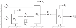
Solution:
We first build the BG model, either manually or using the tools available through 20-sim, with all power bonds labelled, as shown in Figure 11-3. As mentioned, the labels are arbitrary; they merely help bookkeeping of the variables involved without affecting final solution of the system equations. Therefore, the state variables are:  associated with the momenta of the masses and
  displacements of the mechanical springs. The corresponding power bonds to these elements are colour coded (see Figure 11-3). The system equations are ODEs consisting of these state variables. To extract the system equations, we ask two key questions (see section 11.4) and list their corresponding answers, using the power bond labels and causality assignments in terms of BG symbols and , as follows:
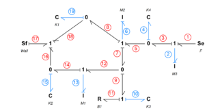
Q1: What does each component/element send to the system?
The inputs to the system are from elements at the boundary of the system associated with bonds 1, 2, 4, 6, 10, 11, 13, 15, 17, and 19, as listed in Table 11-1.
| Power bond label # | System input/relation |
| 1 |  |
| 2 |  |
| 4 |  |
| 6 |  |
| 10 |  |
| 11 |  |
| 13 |  |
| 15 |  |
| 17 |  |
| 19 |  |
Next, we list the relations to answer the second question:
Q2: What does the system send back to the storage components/elements?
Here, we are only interested in storage elements, as shown by colour-coded bonds in Figure 11-3. For example, considering power bond number 2, the system sends an effort signal (or rate of momentum) to the -element representing the mass . Therefore, we can write  . Similarly, considering power bond number 15, the system sends a flow signal (or rate of displacement) to the -element representing the spring . Therefore, we can write
  . Table 11-2 lists all relations corresponding to storage elements.
| Power bond label #(element) | Storage element/relation | Relations, using constraints |
2 ( ) ) |  |  |
4 ( ) ) |  |  |
6 ( ) ) |  |  |
10 ( ) ) |  |  |
13 ( ) ) |  |  |
15 ( ) ) | |  |
19 ( ) ) |  |  |
In the relations listed in the third column of Table 11-2, we used the constraints resulted from 1- and 0-junctions and elements’ constitutive equations, and included the relations from Table 11-1. The final relations are given in bold. Finally, after some manipulations, we can write the system equations in terms of seven state variables in matrix form, as given in Equation (11.4).
(11.4) 
For this example, we consider the electrical system and BG model given in section 7.6 and shown in Figure 7-8. The system has two loops. The number of state variables is three, associated with the storage elements, two inductors and one capacitor.
Solution:
Figure 11-4 shows the BG model with labelled power bonds for this system. The power bonds associated with storage elements, hence state variables, are colour coded.
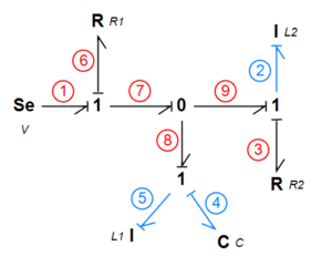
As mentioned, the labels are arbitrary and they merely help bookkeeping of the variables involved without affecting final solution of the system equations. The state variables are:  associated with the momenta of the inductors, and
  , electrical charge of the capacitor. The system equations are ODEs consisting of these variables. To extract the system equations, we ask two key questions (see section 11.4) and list their corresponding answers, using the power bond labels and causality assignments in terms of BG symbols e and f, as follows:
Q1: What does each component/element send to the system?
The inputs to the system are from elements at the boundary of the system associated with bonds
1, 2, 3, 4, 5, and 6, as listed in Table 11-3.
| Power bond label | System input/relation |
| 1 |  |
| 2 |  |
| 3 |  |
| 4 |  |
| 5 |  |
| 6 |  |
Next, we list the relations to answer the second question:
Q2: What does the system send back to the storage components/elements?
Here, we are only interested in storage elements, as shown by colour-coded bonds in Figure 11-4. For example, considering power bond number 2, the system sends an effort signal (or rate of momentum/flux linkage) to the -element representing the inductor . Therefore, we can write  . Similarly, considering power bond number 4, the system sends a flow signal (i.e., current or rate of charge) to the -element representing the capacitor . Therefore, we can write . Table 11-4 lists all relations corresponding to storage elements.
| Power bond label (element) | Storage element/relation | Relations, using constraints |
2 ( ) ) | |  |
4 ( ) ) | |  |
5 ( ) ) |  |  |
Note that  . In the relations listed in the third column of Table 11-4, we use the constraints resulted from 1- and 0-junctions and elements’ constitutive equations, and included the relations from Table 11-3. The final relations are given in bold. Finally, we can write the system equations, after some manipulations, in terms of three state variables in matrix form, as given in Equation (11.5).
(11.5) 
When assigning causality strokes to a BG model, three scenarios may occur [20], [21]. These scenarios are:
– or – element) cannot be assigned with integralAll of these scenarios are legitimate in terms of BG modelling rules, and with red colour-coded causality strokes, 20-sim provides warnings, not errors, for scenarios 2 and 3 as listed above. As mentioned, scenario 1 is desirable and preferred. For this scenario, the system equations can be derived explicitly in terms of state variables as a system of coupled first-order ODEs. The solution of the system of equations provides the answers for the generalized momenta and displacements associated with storage elements. After having the solutions for system equations, we can calculate other desired quantities related to the system.
For the second scenario, the system equations are not independent, i.e., implicit. In other words, the equations related to the storage elements with integral causalities are independent; pertinent state variables can be uniquely calculated by solving these equations, simultaneously. But the equation related to the storage element with derivative causality is not independent; it relates algebraically to the independent equations. Therefore, the related state variable for the element with derivative causality can be calculated using the solution of those of the independent variables. The mathematical dependence of the equation for the derivatively causalled element indicates that the dynamics of the element are related to and defined by the other storage elements in the system. In addition, for the derivative causality case, we may have to force more than one element having non-integral causalities.
For the third scenario, after assigning integral causalities for some of the elements in a definite manner, we face one or more options and have to make choices for one or more elements and arbitrarily assign them with causalities. The resulting system equations are again independent coupled ODEs and can be simultaneously solved to find their solutions. However, during the manipulation, we encounter an implicit equation (or equations) for a particular state variable (or its derivative) which is a function of inputs and itself as well—an algebraic loop. For linear systems/elements, the algebraic-loop situation does not pose a problem; however, for non-linear systems/components, this makes it more difficult to manipulate the equations to find their solutions.
Note that an algebraic loop may occur at several levels and, hence, make it harder to manipulate the equations. This is when, after selecting an assigning causality stroke for an element arbitrarily, further selection(s) should be made to proceed.
For both scenarios, derivative causalities and algebraic loop, the fact that they appear in a BG model is useful information about the system and/or assumptions made for the model, even before solving the resulting equations. In many cases, the modeller can improve the system with additional components, usually of the types of – element.
As mentioned, 20-sim sends warning messages, but no error messages when derivative causalities and algebraic loop exist. The resulted system equations can be solved by solvers available, and the system simulation and design can proceed as usual.
In further sections, we present some examples to demonstrate the derivative causality and algebraic-loop cases.
We consider the BG model shown in Figure 11-5. The colour-coded bonds associated with two inertia -elements are forced, having non-integral causalities or derivative causality. This can be vividly explored by starting assigning causality from -element sending a flow signal to the adjacent 1-junction. Therefore, all other connecting bonds to this 1-junction should have their causality strokes at the ports connecting to this 1-junction. This requirement forces the associated -element to have a derivative causality, or sending effort signal, instead of receiving it for being integrally causalled, to the 1-junction. Similarly, the -element  is forced to have derivative causality. As a result, the momenta of these two -elements (i.e. and ) will depend on the remaining storage elements, i.e., -element
  and -element , and can be calculated having the corresponding solutions for – and – elements. For further reading, consult with references cited as [5], [20], [21], and [30].
As mentioned, in 20-sim a warning message appears on the screen when derivative causality exists in the BG model. But the software solver tools take care of this and solve the system equations. This capability is useful for practical applications in design of the systems.
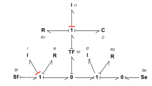
We consider the BG model shown in Figure 11-6. Starting with the process of assigning causalities, we realize that the colour-coded bonds can’t be integrally assigned and present options. In other words, to proceed further with assigning causalities to the whole system’s BG model, we require to make a selection arbitrarily. Usually, the selection can be more easily made with -elements, since it can be assigned with neutral causality. For example, if we select the element  and assign causality stroke to it such that it sends a flow signal to the adjacent 1-junction, then the remaining bonds’ causality strokes can be assigned, as shown colour coded in Figure 11-7. Alternatively, element
  or
or  could be selected as an option. The corresponding BG models and related assigned causalities are shown in Figure 11-8 and Figure 11-9, respectively.
For further reading, consult with references cited as [5], [20], [21], and [30].
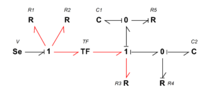
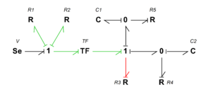
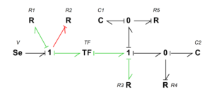
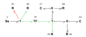
As mentioned, in 20-sim, a warning message appears on the screen when algebraic loop causality exists in the BG model. But the software solver tools take care of this and solve the system equations. This capability is useful for practical applications in design of the systems.
Thermal systems are unique in terms of BG modelling. They are closely analogous to electrical systems. In practice, to analyze thermal systems, we use this analogy to build models as thermal networks, similar to electrical networks, [39], [40].
Considering heat conduction through a solid slab, e.g., the temperature difference  (analogous to voltage) and heat flow rate
  (analogous to electrical current) satisfy
  . The quantity
  (analogous to electrical resistance) is thermal resistance with dimension [K/W], in
  , where,
  is the length across which the applies; is the cross-sectional area for heat flow, and is the thermal conductivity of the material. Intuitively, this analogy suggests to consider temperature as the effort and the heat flow rate as the flow when building BG models for thermal systems. With this assumption at hand, the product (
 ) would be considered as power variables, or the dimension of this quantity should be as of that for power. However, close examination of the dimension for the product () gives its dimension as
 ![[(T\dot Q_{th})] = K \cdot W](https://pressbooks.bccampus.ca/engineeringsystems/wp-content/ql-cache/quicklatex.com-653b673f38ea3f787dec941dcc3b5cf3_l3.svg "Rendered by QuickLaTeX.com") , or
, or  . Therefore, according to BG modelling rules, we cannot accept temperature and heat flow rate as conjugate power variables. This discrepancy leads us to call such a BG model a pseudo bond graph (pseudo BG), for which temperature is the effort and heat flow rate is the flow. This is acceptable as far as the thermal system is the only system involved and the modeller is aware of the fact that the “power” variables are not defined fully and correctly in the related thermal pseudo BG model. However, for multi-domain systems, the exchange of power between a thermal sub-system part and other domains of the system becomes problematic.
The solution to this challenge comes from the second law of thermodynamics, which guides us to consider the flow in the BG model as the entropy rate, instead of heat flow rate. Recall that entropy is a state function, and for a reversible system, we have the relationship  for exchange of heat
  and entropy
  using temperature , [41]. Therefore, the heat flow rate is
  . The dimension of
  , the entropy rate, is then [
 ]. Therefore the dimension of the power variables, or (
 ) is [
 ], as it should be; hence, we can accept the temperature as the effort and entropy rate as the flow (or entropy as displacement) in BG model for a thermal system. Table 11-5 shows the variables involved in Pseudo BG and BG models for thermal systems.
| Model | Effort | Flow | Power | System |
|---|---|---|---|---|
| Pseudo BG | temperature | heat flow rate | ill-defined | single thermal domain |
| BG | temperature | entropy rate | defined | multi-domain |

1
References | |
| [1] | H. M. Paynter, Analysis and Design of Engineering Systems, Boston, MA: MIT Press, 1961. |
| [2] | Ronald Zamora-Musa and Jesus Coba, “Trends in modeling and simulation in the automotive industry concerning the bond graph framework,” International Journal of Engineering & Technology, vol. 7, pp. 160-163, 2018. |
| [3] | Controllab, Introduction to 20-sim, Accessed: 2020. [Online]. Available: https://www.20sim.com/overview/introduction/ |
| [4] | M. Tiller, Introduction to Physical Modeling with Modelica, Kluwer Academic Publishers, 2001. |
| [5] | Charles M. Close and Dean K. Frederick, Modeling and Analysis of Dynamic Systems, 3rd ed., Wiley, 2015. |
| [6] | Modelica Association, Modelica Tools, Accessed: 2020. [Online]. Available: https://www.modelica.org/tools. |
| [7] | J. Lagrange, Méchanique Analytique; English, translated and edited by Auguste Boissonnade and Victor N. Vagliente., Boston: Kluwer Academic Publishers, 1997. |
| [8] | P. Hamill, A Student’s Guide to Lagrangians and Hamiltonians, Cambridge University Press, 2013. |
| [9] | E. Khutoryansky, Euler-Lagrange equation explained intuitively – Lagrangian Mechanics (Nov. 18 2018).[Online Video]. Available: https://www.youtube.com/watch?v=EceVJJGAFFI |
| [10] | J.E. Marsden and T.S. Ratiu, Introduction to Mechanics and Symmetry – A Basic Exposition of Classical Mechanical Systems, 2nd edition, Springer, 2002. |
| [11] | Goldstein, H., Poole Jr, C.P., and Charles, P, Classical Mechanics, 3rd ed., Pearson, 2013. |
| [12] | E. Kreyszig, Advanced Engineering Mathematics, 10th ed., Wiley, 2011. |
| [13] | Tom W.B Kibble and Frank H. Berkshire, Classical Mechanics, 5th ed., Imperial College Press, 2014. |
| [14] | W. Hamilton, “On a General Method in Dynamics,” Philosophical Transactions of the Royal Society, pp. Part I, pp. 95-144, Part II, pp. 247-308, 1834,1835. |
| [15] | K. Cassel, Variational Methods with Applications in Science and Engineering, Cambridge University Press, 2013. |
| [16] | W. Greiner, Classical Mechanics, Springer-Verlag, 2010. |
| [17] | R. d. Callafon, , MAE courses. [Online]. UCSD Available: http://maecourses.ucsd.edu/callafon/labcourse/lecturenotes/Lagrange_Handout.pdf. [Accessed Oct., 2019]. |
| [18] | M. Tabatabaian, Tensor Analysis for Engineers, 2nd ed. Mercury and Learning Information, 2021. |
| [19] | N. A. Lemos, “Atwood’s machine with a massive string,” European Journal of Physics, vol. 38, no. 6, Sep., 2017. doi: arXiv:1710.01263V1. |
| [20] | Dean C. Karnopp, Donald L. Margolis, and Ronald C. Rosenberg, System Dynamics: Modeling and Simulation of Mechatronic Systems, 4th ed. Wiley Publishing, 2006. |
| [21] | S. Das, Mechatronic Modeling and Simulation Using Bond Graphs, 1st ed. Boca Raton: CRC Press, 2009. |
| [22] | B. T. Forbes, Engineering Systems Dynamics: A Unified Graph-Centered Approach, 2nd ed. CRC Press., 2007. |
| [23] | James L. Meriam, L. G. Kraige, J. N. Bolton, Engineering mechanics: Dynamics, 8th Edition, Wiley, 2015. |
| [24] | Charles Alexander and Matthew Sadiku, Fundamentals of Electric Circuits, 7th ed. McGraw-Hill Education, 2020. |
| ED.[25] | NASA, “Wheatstone Bridge Circuit,” N. Hall, Ed. 2015. [Online]. Available: https://www.grc.nasa.gov/WWW/K-12/airplane/tunwheat.html. [Accessed 2020]. |
| [26] | I. Shames, Mechanics of Fluids, 4th ed. McGraw-Hill, 2002. |
| [27] | F. M. White, Fluid Mechanics, McGraw-Hill, 2015. |
| [28] | M. Tabatabaian, CFD Module: Turbulent Flow Modeling, Mercury Learning and Information, 2015. |
| [29] | Yilei Li, Zhencai Zhu, and Guoan Chen, “Bond Graph Modeling and Validation of an Energy Regenerative System for Emulsion Pump Tests,” The Scientific World Journal, vol. 2014, pp. 1-12, 2014. |
| [30] | J. A. Kypuros, System Dynamics and Control with Bond Graph Modeling, CRC Press, 2013. |
| [31] | N. S. Nise, Control Systems Engineering, 8th ed., John Wiley & Sons, 2019. |
| [32] | P. Gawthrop and L. Smith, Metamodelling: For Bond Graphs and Dynamic Systems, Prentice Hall, 1996. |
| [33] | W. Borutzky, “Bond Graph Modelling and Simulation of Mechatronic Systems- An Introduction into the Methology,” in 20th Europeann Conference on Modelling and Simulation, Bonn, 2006. |
| [34] | Fan, Zhun, et. al., “Exploring Multiple Design Topologies Using Genetic Programming And Bond Graphs,” in GECCO 2002: Proceedings of the Genetic and Evolutionary Computation, New York, 2002. |
| [35] | G. Strang, Introduction to Applied Mathematics, Wellesley-Cambridge Press, 1986. |
| [36] | K. Ogata, Modern Control Engineering, 5th ed. Pearson, 2009. |
| [37] | H. W. Bode, Network Analysis and Feedback Amplifier Design, D. Van Nostrand, 1945. |
| [38] | B. York, “Frequency Response and Bode Plots,” 2009. [Online]. Available: https://web.njit.edu/~levkov/classes_files/ECE232/Handouts/Frequency%20Response.pdf. [Accessed 2020]. |
| [39] | John H. Lienhard V and John H. Lienhard IV, A Heat Transfer Textbook, 5th ed. Cambridge, Massachusetts: Phlogiston Press, 2019. |
| [40] | Y. A. Cengel, Heat Transfer: A Practical Approach, McGraw-Hill, 2002. |
| [41] | M. Tabatabaian and ER.R.K. Rajput, Advanced Thermodynamics: Fundamentals, Mathematics, Applications, Mercury Learning and Information, 2017. |
| [42] | G. Romero, et. al., “Kinematic Analysis of Mechanism By Using Bond-Graph Language,” in 20th European Conference on Modelling and Simulation, 2006. |
2
This page lists major changes to this book with major changes marked with a 1.0 increase in the version number and minor changes marked with a 0.1 increase.
| Version | Date | Change |
| 1.0 1.1 | October 2021 May 2022 | PressBook Created Typos, Figures, some Exercises |
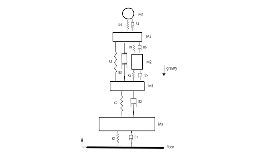