Chapter 3: Climate Responsive Design
Jens Voshage
Data driven climate responsive design is an exciting new place to explore. The idea to work with climate data has been common practice in energy consulting and modeling for some time now. It makes sense to use the same kind of data to help understand the climate and make this information intuitively accessible to the right-brain-leaning architecture and landscape designer community. Especially as feedback loops and turn-around times for project decisions in early predesign and schematic design are tight, sometimes days, sometimes hours; it can be hard, even impossible to involve special consultants for those early, but for building performance, crucial decisions. In those “sketch” phases you will be making decisions on the building location on the site, orientation, program distribution, aperture ratio etc., all these metrics have huge impact on comfort and energy performance (thus carbon performance).
In this context the next logical step is to connect the world of GIS with the world of BIM to draw conclusions and define boundary conditions from a larger geographic scale. Both GIS (Geographic Information Modeling) and BIM (Building Information Modeling) use a similar methodology as that they both use a digital geometric twin of environmental features connecting it with tables of alphanumeric data. Along the full bandwidth from rural to urban transects, drawing information from GIS to create context is very reasonable as GIS concerns itself with capturing and mapping the natural world as well as the human made environment. Both approaches (BIM, GIS) have developed from within different siloed specialty disciplines (geography, architecture, engineering), generated their own file formats and software package, so the main challenge is the interface to exchange data back and forth.
This Chapter is meant to supplement the “in-situ” experiences, observations, and analysis. It is written to serve as a hands-on inspiration and recipe collection. This type of proposed and described resource mapping lends itself to holistic recognition of risk and solutions in ecological context-sensitive design and place-based stewardship. The hope is to support bigger-picture design methodologies mentioned in other chapters like the Living Building Challenge, Regenerative Design, Permaculture.
The Changing Climate System and Ecology
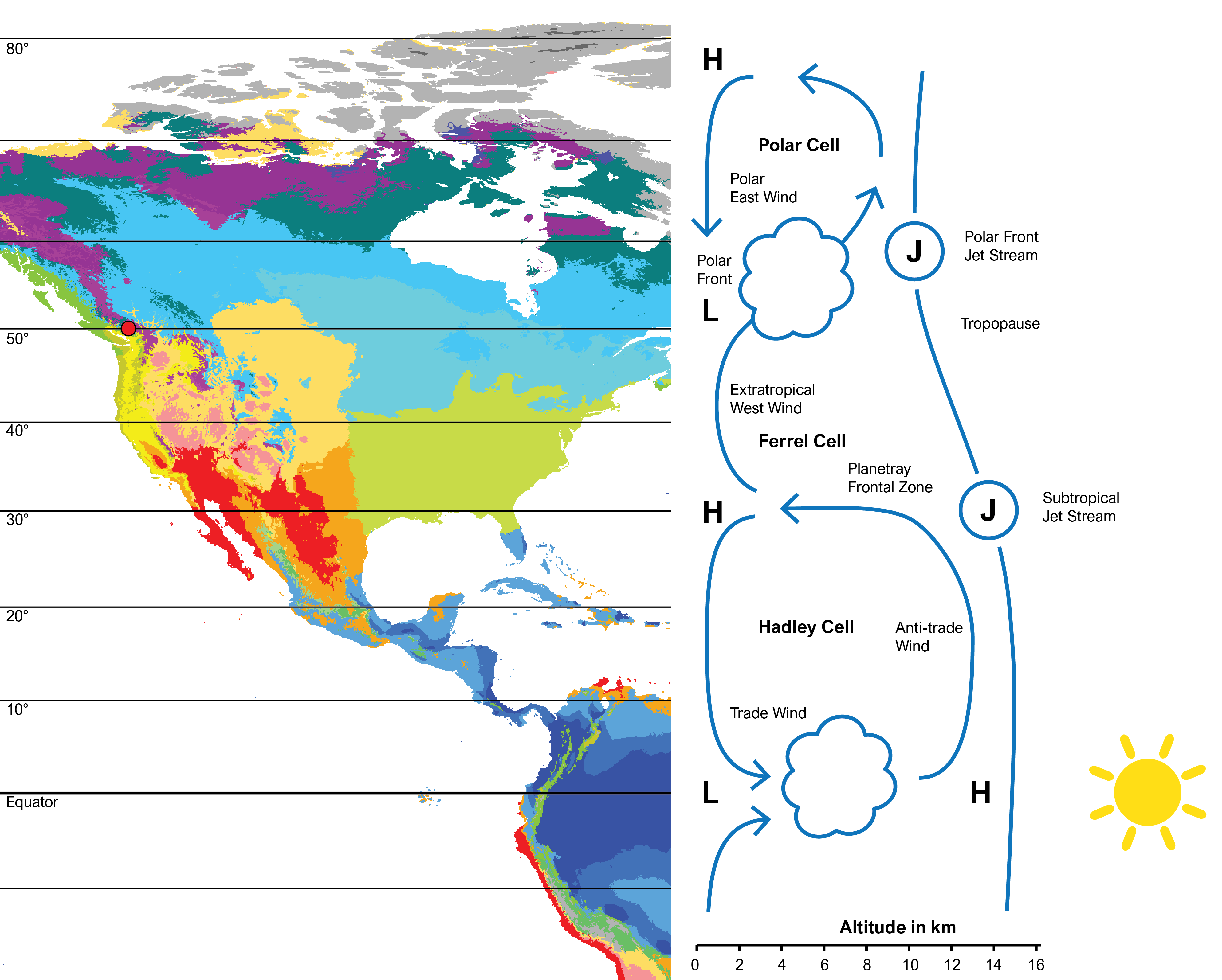
The climate system receives its energy from the radiation of our sun (electro-magnetic energy) and to a lesser degree from the tidal effects of the moon (gravitational energy) and the earth’s core (thermal and gravitational energy). Without the solar driven planetary energy balance with all its feedback loops no life on earth would be possible today. The Gaia hypothesis proposes feedback loops and interactions between the lithosphere, the atmosphere, and the biosphere, which created and stabilized those favorable climate conditions and ecoregions that helped our specie’s living conditions and cultures to thrive and develop over the last 10,000 and more years (Holocene[1]).
Ecology in this context is meant to describe those complex interacting systems of life with the physical world (You can use The Deep Time Walk as a powerful tool to connect with the evolution of those well tuned and balanced ecological systems which created conditions conducive to life[2]).
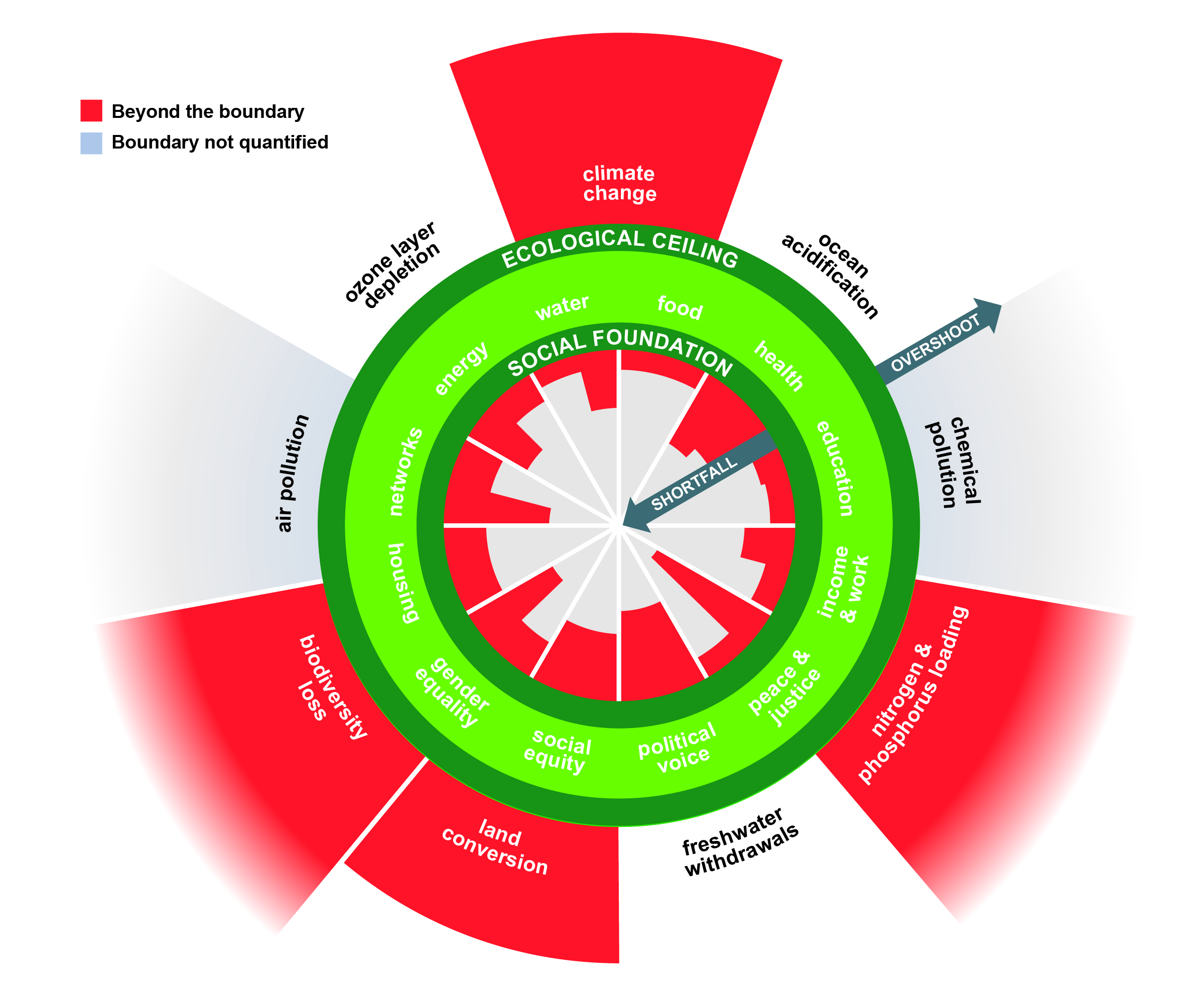
Since the discovery of fossil sunlight (coal, oil, and gas) some 200ish years ago this balanced and stable climate era gave way to a new and unpredictable climate epoch that is called the Anthropocene. This era is named due to rapid and strong human interventions to our earth’s systems by the means of sinking carbon (CO2) from the conversion of subterranean fossil sunlight into thermal and other forms of energy into the atmosphere, changing life’s nutrient cycles (nitrogen, phosphorus), polluting with chemical compounds that never existed, and changing biodiversity, water, and energy cycles through land surface conversion amongst others. The doughnut diagram below, that was perceived for the book Doughnut Economics by Kate Raworth (Figure 1) helps to visualize the anthropogenic impacts on the ecology. The observed changes in weather patterns and weather extremes and the shifting climate averages are just one of the aspects of imbalance of a previous relatively stable ecological system. Of all anthropogenic induced changes of subsystems, it is probably, at least for now the climate that has the most impact on building design decision making.
Climate Elements and Climate Factors
“Climate is what we expect, weather is what we get.”
Mark Twain
A climate element is a parameter which describes the climate at a specific location and can be measured via a weather station. Common climate elements are dry bulb temperature, relative humidity, solar radiation (electromagnetic energy per area), wind direction, wind speed, cloud coverage, precipitation, snow depth etc. Climate factors are terrestrial situations influencing the mesoclimate (regional) or microclimate (site). Climate factors are relatively stable, they can include latitude, altitude, relief, water and land patterns, land use (type of vegetation, human land use e.g. creating urban heat island effect)
Climate in Architectural Design Decision Making
The climate needs to be considered for global warming mitigation through minimising construction and operations impacts to greenhouse gas emission contributions and land use degradation. We all know that. Tools for minimizing material carbon emissions (embodied carbon) as well as operational carbon emissions (mostly via combustion of fossil and biomass) will be discussed in later chapters. Below are some examples of methodologies toward post carbon construction.
- Life Cycle Assessment
- Carbon Accounting
- Zero Carbon Building Operations
- Passive House
Our local climate conditions used to define how we lived, how we moved around, what food was available to grow, to preserve and store over time, our activities were determined by the seasons, and vernacular architecture was the response to provide shelter and comfort for a specific local climate with specific local resources available.
The fossil fuel blip seduced us to build as if there is no climate. Many buildings tended to look the same worldwide for a period from the 1950ies on. No matter how harsh the conditions, machines were used to maintain comfort through brute-force heating, cooling and fresh air etc.
It is those local ambient climate conditions that we now must use again to drive design strategies toward passive comfort, passive energy, and passive resilience (passive solar orientation and aperture, solar PV, solar DHW, wind energy, wind and stack driven fresh air ventilation, night-flush cooling, independence from machines for comfort and safety) without reliance on fossil energy carriers as these energy dense marvels of stored sunlight will either naturally decline or intentionally phased out.
For the purpose of design and construction philosophy that is in sync with the idea of mitigation and adaptation to the ever changing current and future climate and energy conditions and it’s posed challenges the following chapters want to demonstrate methods and tools to visualize, simulate, analyze climate and site related conditions, and apply conclusions to your building design intents.
Analyzing the Local Climate for Informed Decision Making Climate Data
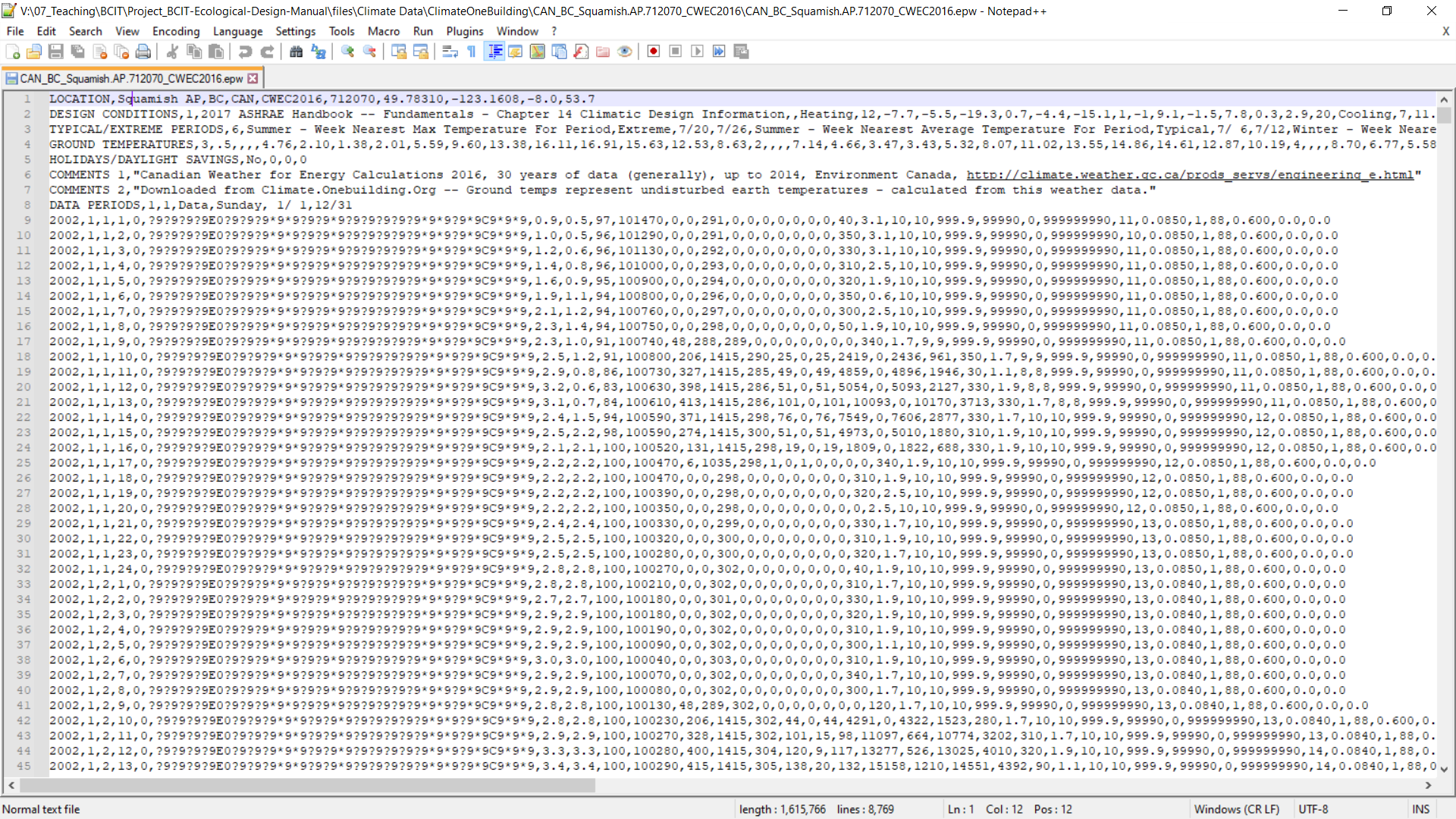
In the world of building simulation, you will come across confusing terminology. If engineers and modelers talk about a specific set of typical average climate data, they will quite often call it a weather file. Local weather files for building design analysis and energy simulation are typically structured as an annual data set that includes 8760 entries for many of the mentioned climate elements (one entry per parameter for every hour of the year). The most common file format is an EPW file. The EPW format was developed by the US Department of Energy to be a standard weather data format. This file format contains up to 35 core climate elements formatted to be used originally in conjunction with the open-source energy modelling software EnergyPlus[3], thought most building simulation software will be able to read EPW files. EPW is a quasi standard for climate data exchange. Quite often various climate element columns contain no data or gibberish. Most often the precipitation data has been omitted. The climate data is collected over decades and synthesized to represent typical average conditions for that time frame. Files are sometimes named TMY which stands for Typical Meteorological Year. TMY2 represents the years 1961 – 1990 and TMY3 1991 – 2005. In Canada you might come across the abbreviation CWEC (Canadian Weather Year for Energy Calculation) which uses similar algorithms to derive typical values as the TMY approach.
EPW Weather File Dictionary
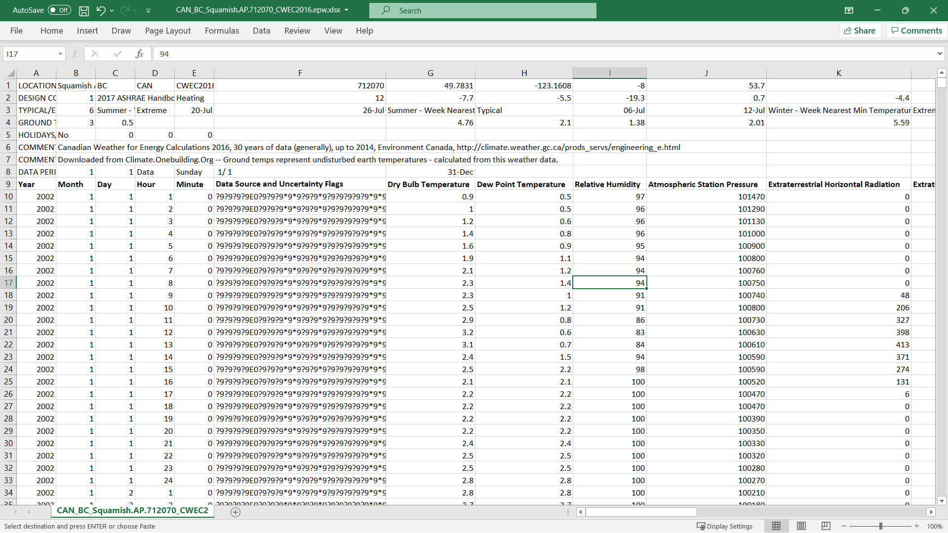
At bigladder software[4] you can find a comprehensive documentation of terminology and units used in the EPW for various climate elements. The table below gives you a glance overview of the content.
| Data Field | Unit |
| Year | |
| Month | |
| Day | |
| Hour | |
| Minute | |
| Data Source and Uncertainty Flags | |
| Dry Bulb Temperature | °C |
| Dew Point Temperature | °C |
| Relative Humidity | % |
| Atmospheric Station Pressure | Pa |
| Extraterrestrial Horizontal Radiation | Wh/m² |
| Extraterrestrial Direct Normal Radiation | Wh/m² |
| Horizontal Infrared Radiation Intensity | Wh/m² |
| Global Horizontal Radiation | Wh/m² |
| Direct Normal Radiation | Wh/m² |
| Diffuse Horizontal Radiation | Wh/m² |
| Global Horizontal Illuminance | lux |
| Direct Normal Illuminance | lux |
| Diffuse Horizontal Illuminance | lux |
| Zenith Luminance | Cd/m² |
| Wind Direction | N=0; E=90; W=270 |
| Wind Speed | m/sec |
| Total Sky Cover | tenth of coverage |
| Opaque Sky Cover | tenth of coverage |
| Visibility | visibility in km |
| Ceiling Height | m |
| Present Weather Observation | 0 or 9 (0=yes; 9=no) |
| Present Weather Codes | |
| Precipitable Water | mm |
| Aerosol Optical Depth | |
| Snow Depth | cm |
| Days Since Last Snowfall | |
| Albedo | ratio |
| Liquid Precipitation Depth | mm |
| Liquid Precipitation Quantity | hr |
Sources for Weather Files
Here are a few sources for public domain and as well commercial global and Canadian climate data sets:
- https://energyplus.net/weather
- http://climate.onebuilding.org
- https://climate.weather.gc.ca/prods_servs/engineering_e.html
- https://energy-models.com/equest-and-epw-files-worldwide
- http://weather.whiteboxtechnologies.com/
- https://meteonorm.com/en/
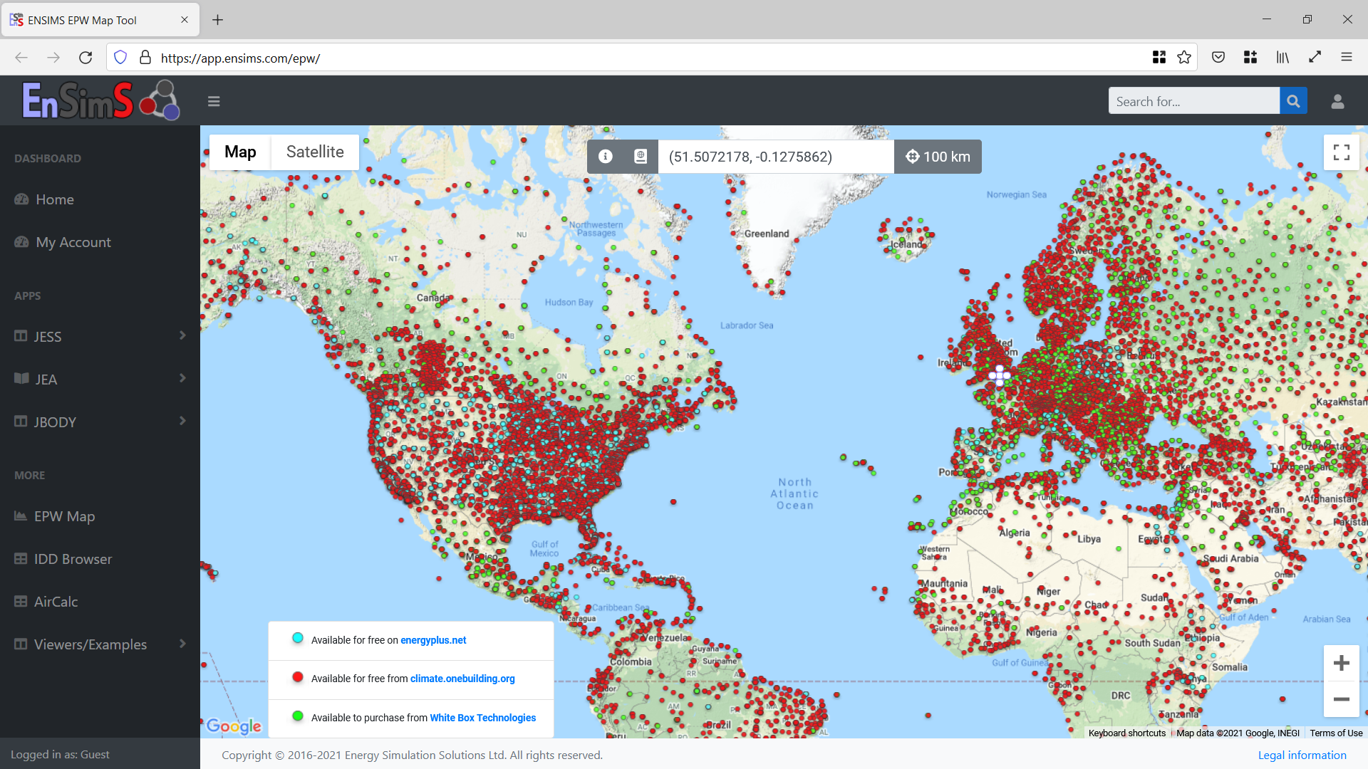
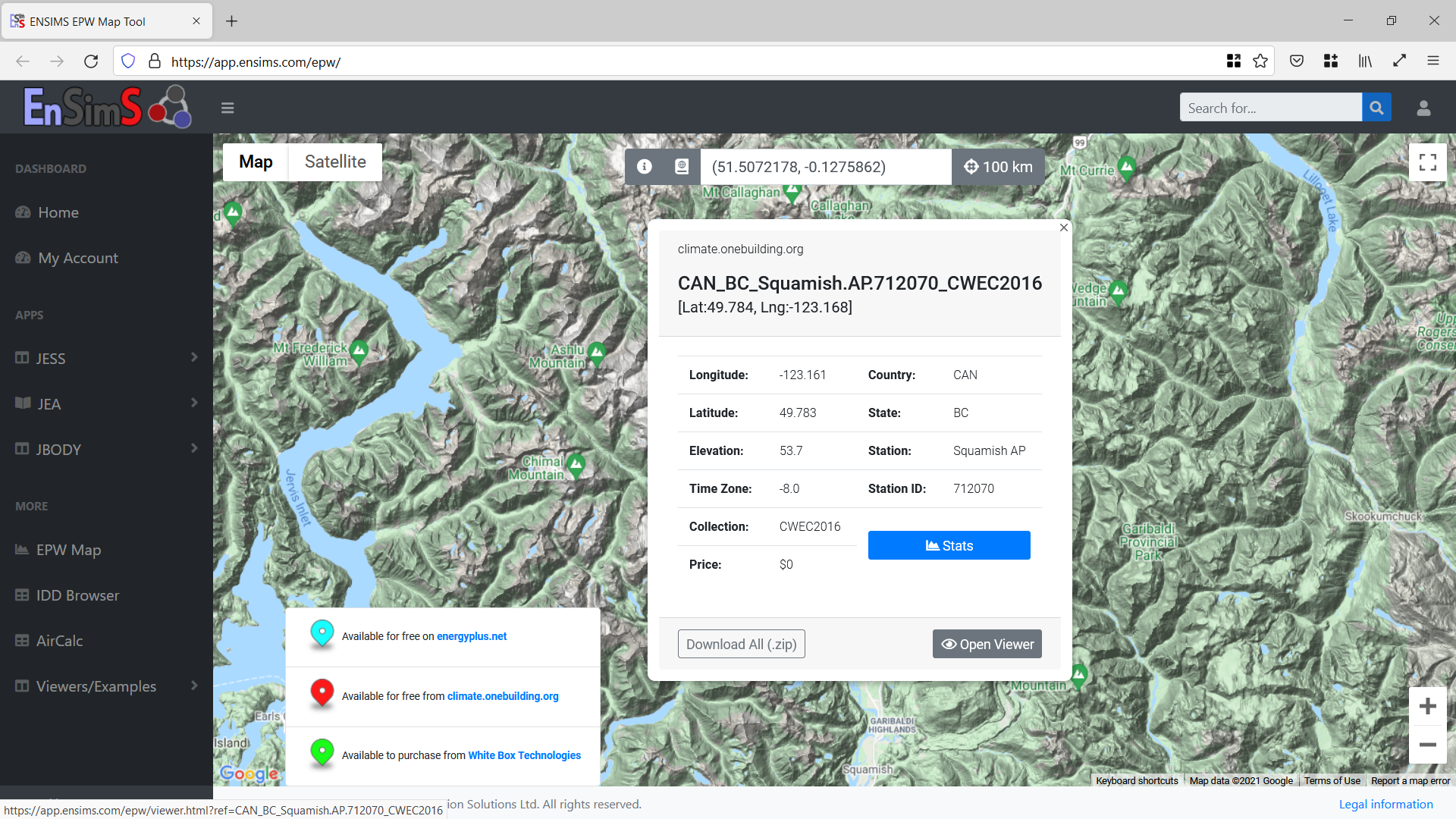
Some of the free data sources have been consolidated on mapping user interfaces to allow for more convenient access. The app.ensims.com site lets you graphically visualize the most important aspects of the EPW data right within the same interface after selecting the desired location pin on the map.
Creating and Editing EPW Weather Data Files
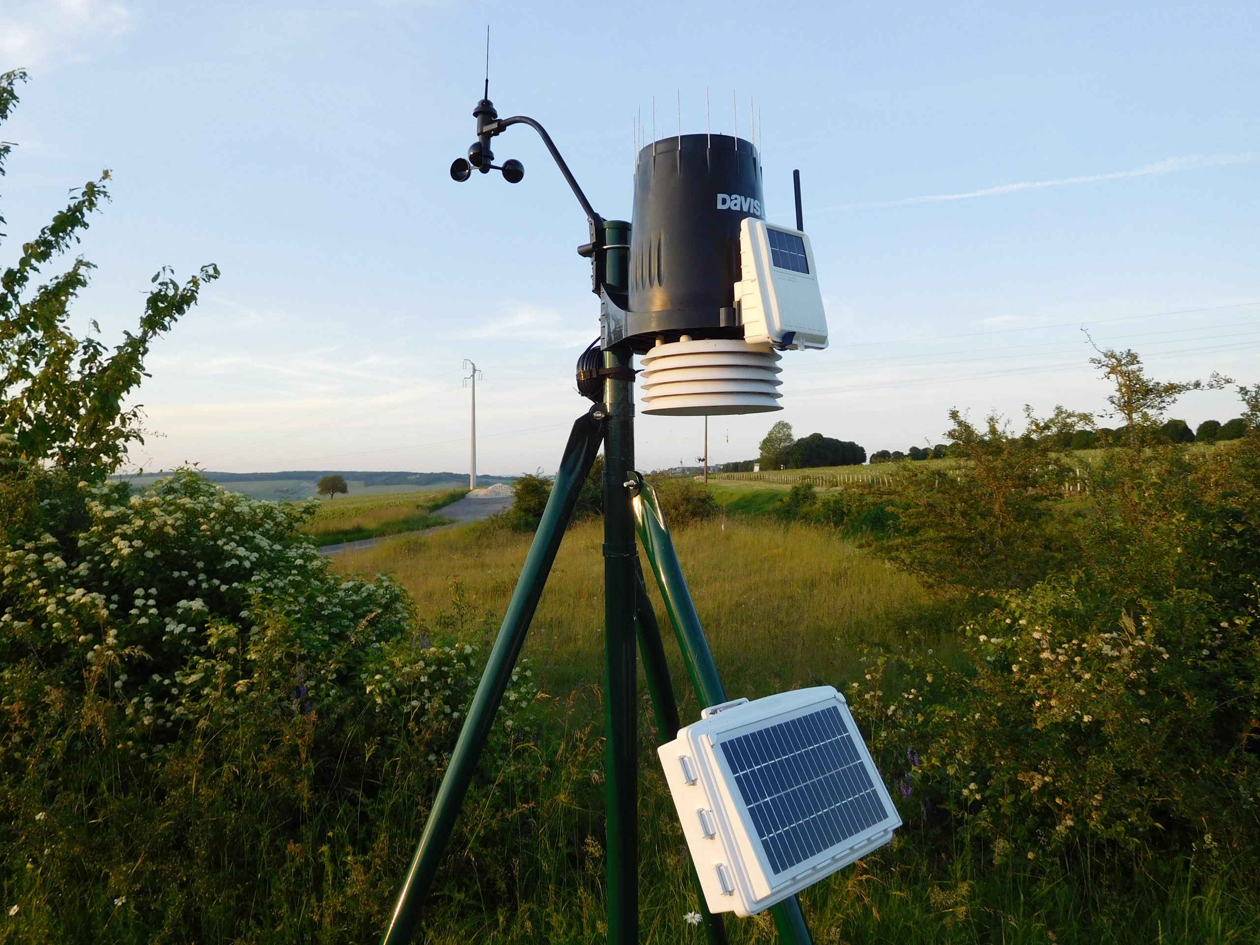
If you believe that your project site has a unique microclimate, and it would be useful to create your own weather file you should at least work from a full year collection cycle from your site weather station. Weather stations that allow for live monitoring and cloud data collection can be rented relatively inexpensively.
To then create your own EPW you should start with an existing file that is as close as possible to your custom location. Make sure that you convert your collected data to the right time steps (hourly) as required for EPW. Make feasible assumptions of how your one year measurement might be representative for the average climate, use the measured data for the existing file from the same year for calibration.
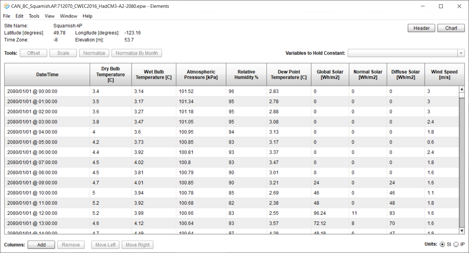
The free and open-source EPW editor Elements[5] bigladder software allows you to create new weather files based on your own measurements, or edit data points individually or batch offset, scale or normalize the existing data sets.
Climate Data Visualization and Analysis
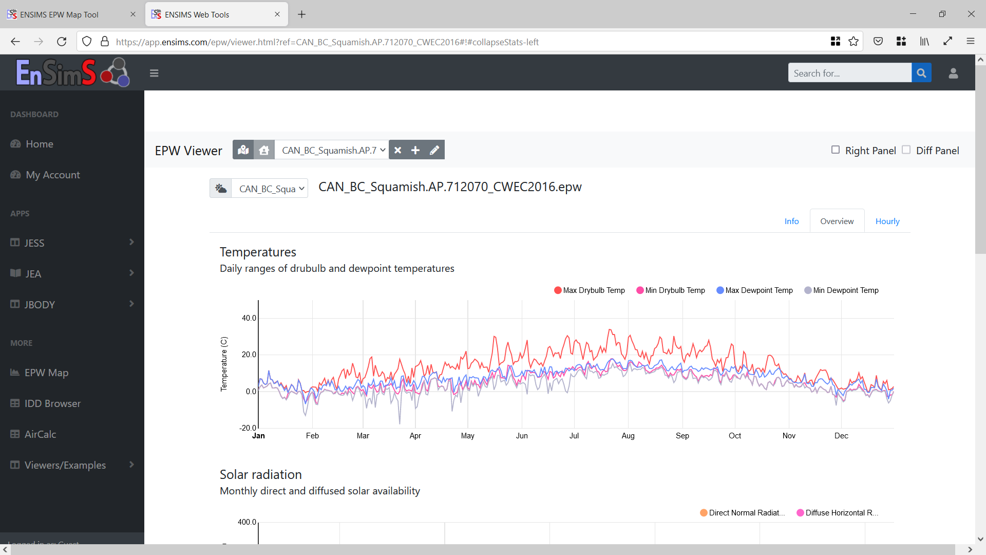
Weather files are typically used by energy modelers to predict operational building performance via dynamic energy modeling software, but we can also visually and interactively explore these huge data files beyond looking at columns and rows in Excel using specialized tools. As architects, or maybe just being human, this type of data can be much better computed in our brains when presented visually rather then alphanumerically.
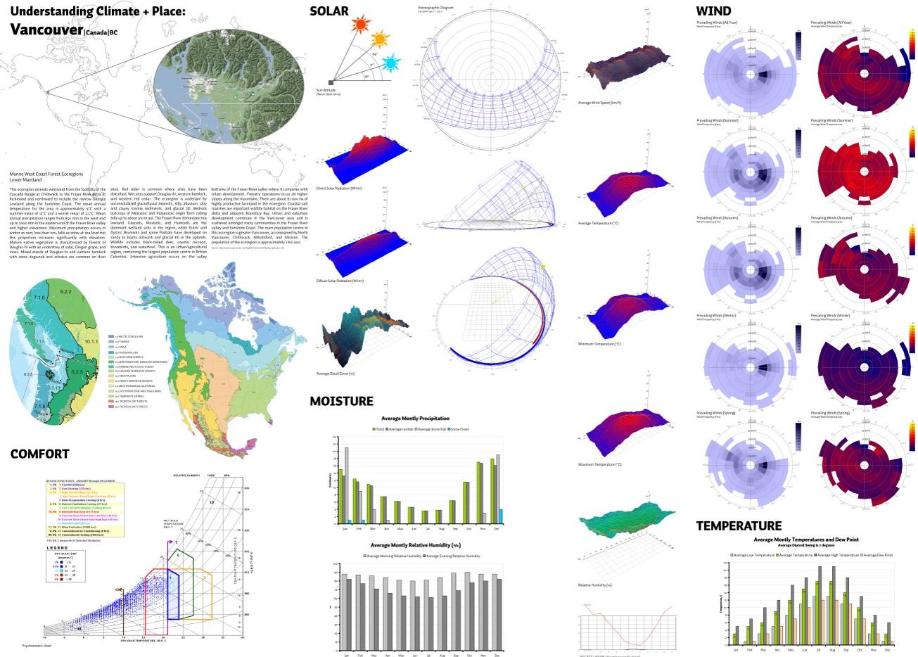
The intend to visualize climate data is to allow the design team to do blink assessments on design strategies without reverting to time consuming computer simulations. The best format to communicate this information is a poster layout that would be omnipresent in the designer’s studio.
There are many web-based and standalone applications that help us to see the forest for the trees while looking at big tables of weather data. Some are exemplary mentioned in this chapter, others are listed in the Tools and Databases section at the end of this chapter.
For the purpose of this manual these are the two weather files that are being used for the demonstrations below:
- CAN_BC_Squamish.AP.712070_CWEC2016.epw
- CAN_BC_Squamish.AP.712070_TMYx.2004-2018.epw
Andrew Marsh – Data View 2D
Available via http://andrewmarsh.com/software/data-view2d-web/
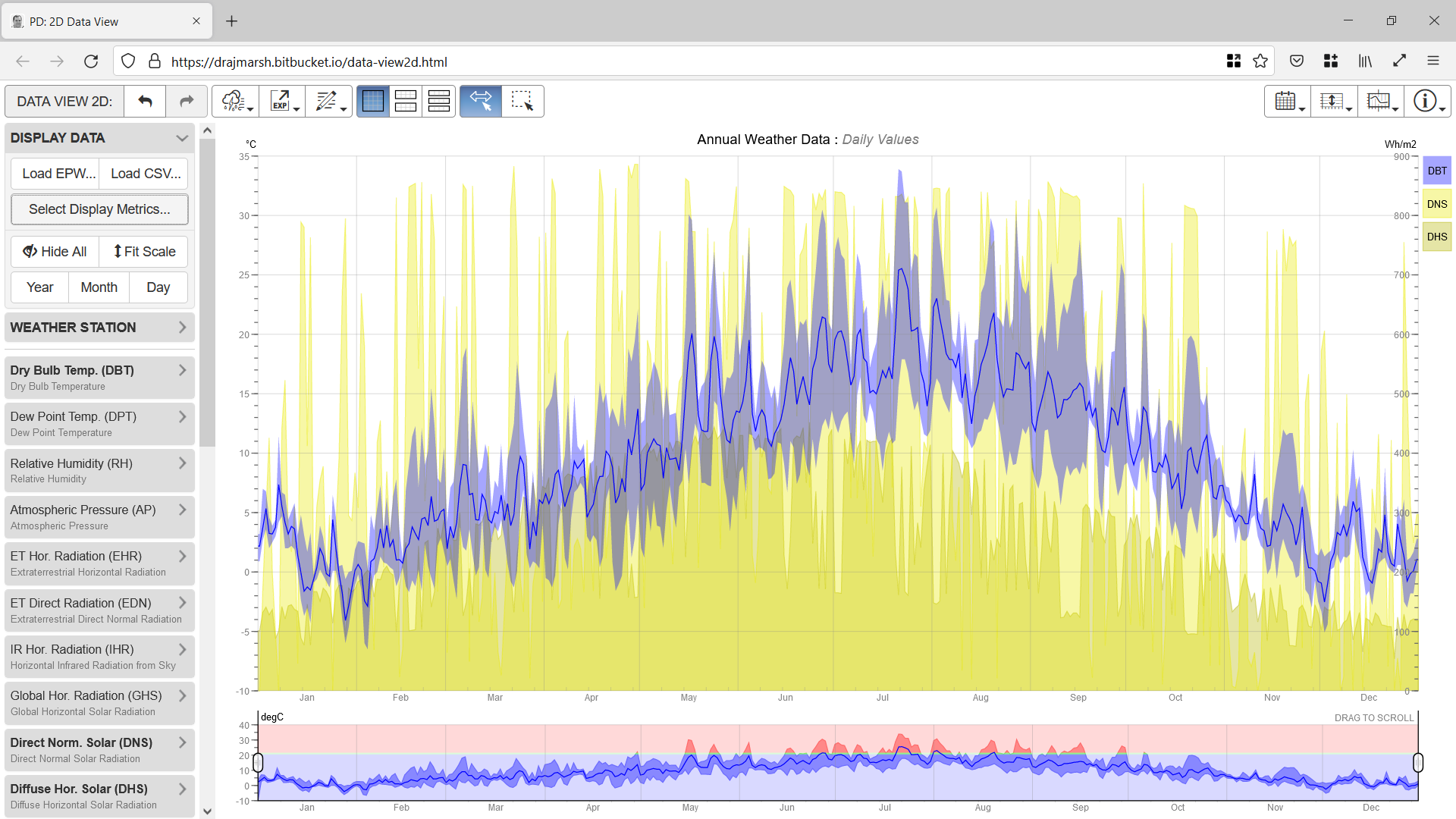
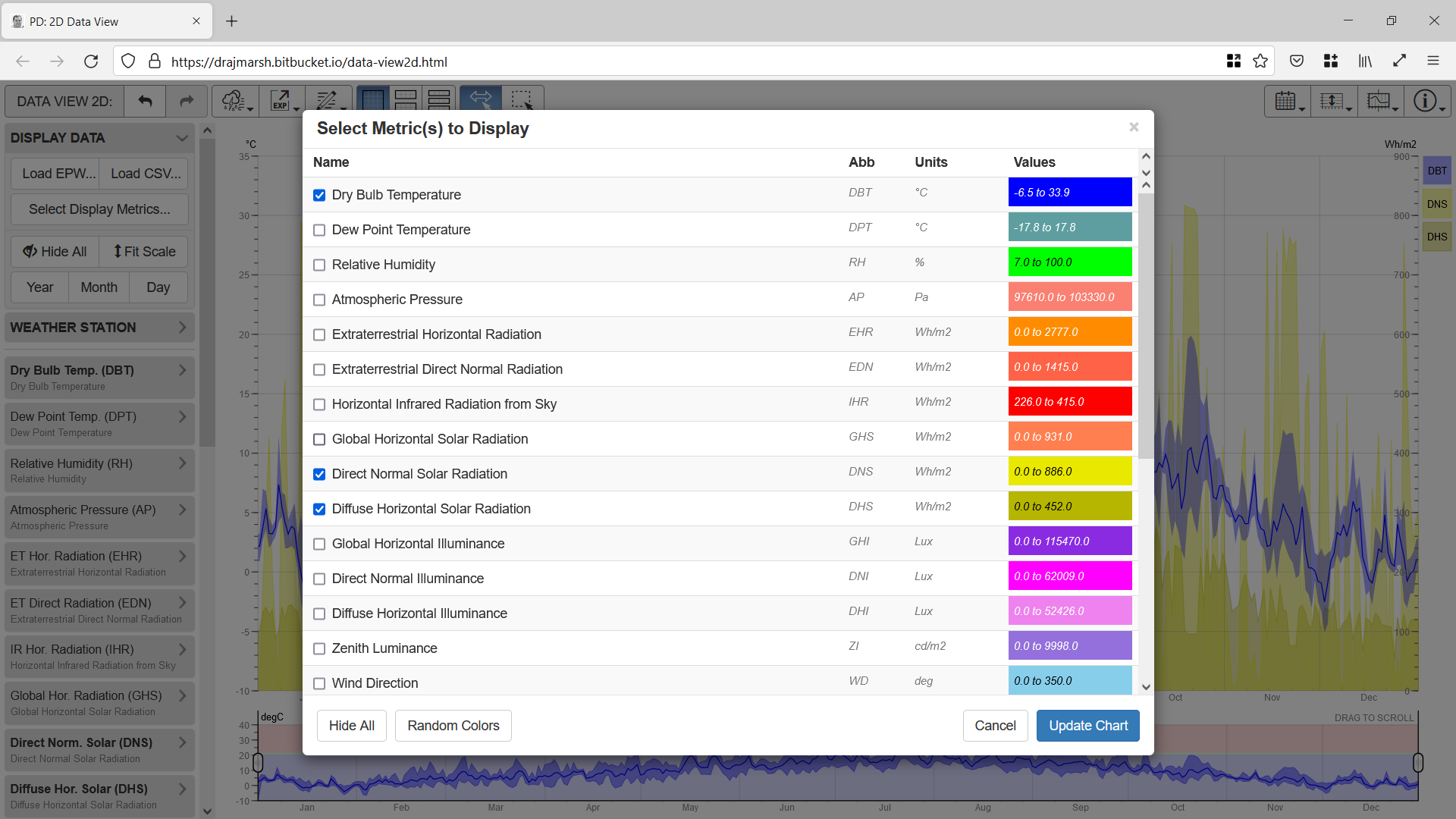
“This web app displays annual hourly weather or analysis data in a series of synchronised charts. It can read EnergyPlus weather data (EPW) as well as EnergyPlus output data files (CSV). As both these formats contain large amounts of hourly data, it lets you select which metrics to view and compare as well as the date range over which to render them.”
URL: http://andrewmarsh.com/software/data-view2d-web/; Website title: Data View 2D; Date accessed: November 17, 2021
Andrew Marsh – Weather Data
Available via http://andrewmarsh.com/software/weather-data-web/
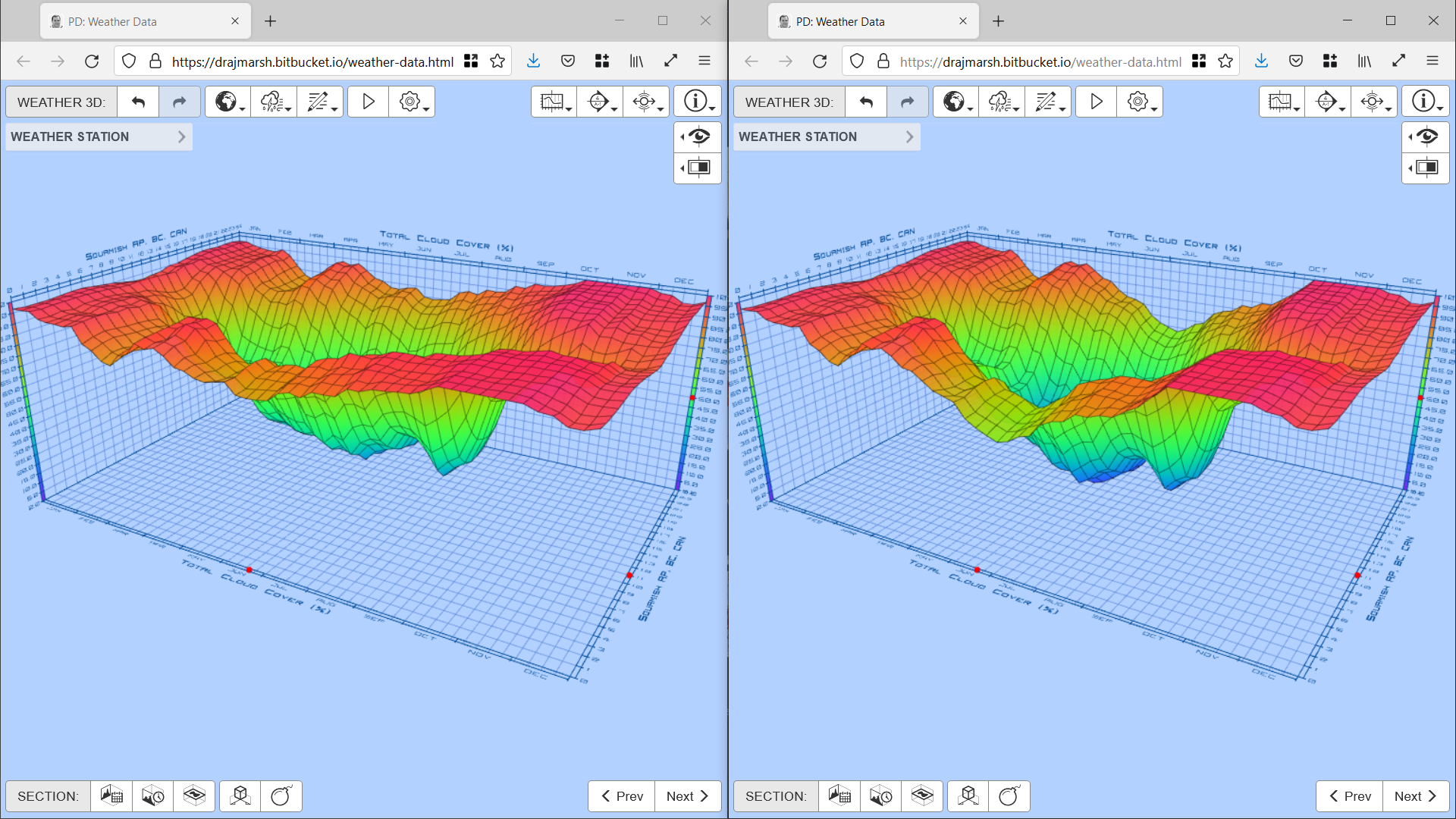
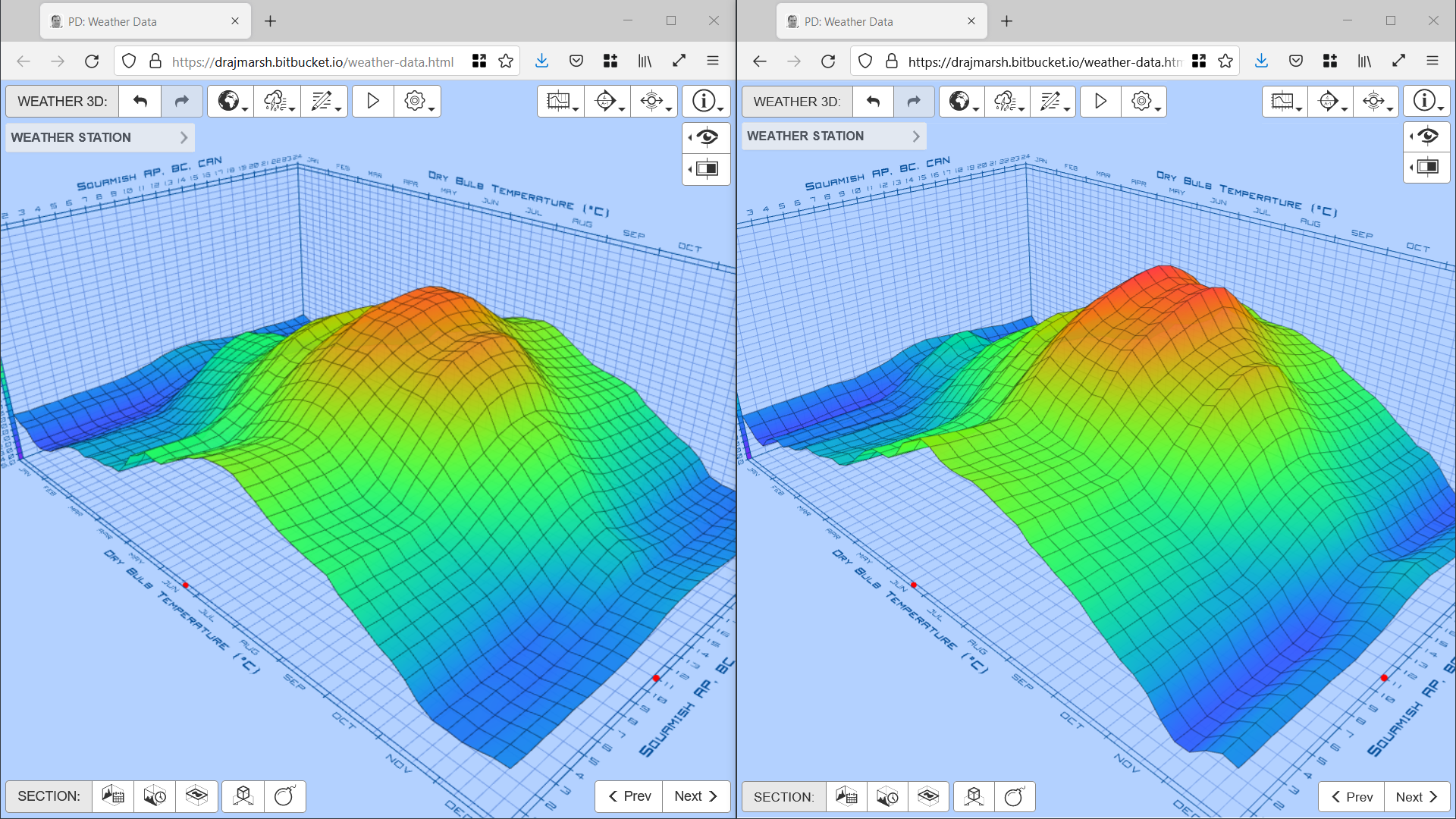
“This web app lets you load and display EnergyPlus weather data in a 3D graph with data averaging and animated sectioning. It maps the full range of weather data metrics against day of the year and hour of the day to create an undulating 3D surface plot. You can interactively adjust the displayed metric, the graph size and scale, section planes and data averaging parameters. Simply drag&drop a .EPW file anywhere in the browser windows and you are ready to go.”
URL: http://andrewmarsh.com/software/weather-data-web/; Website title: Weather Data; Date accessed: November 17, 2021
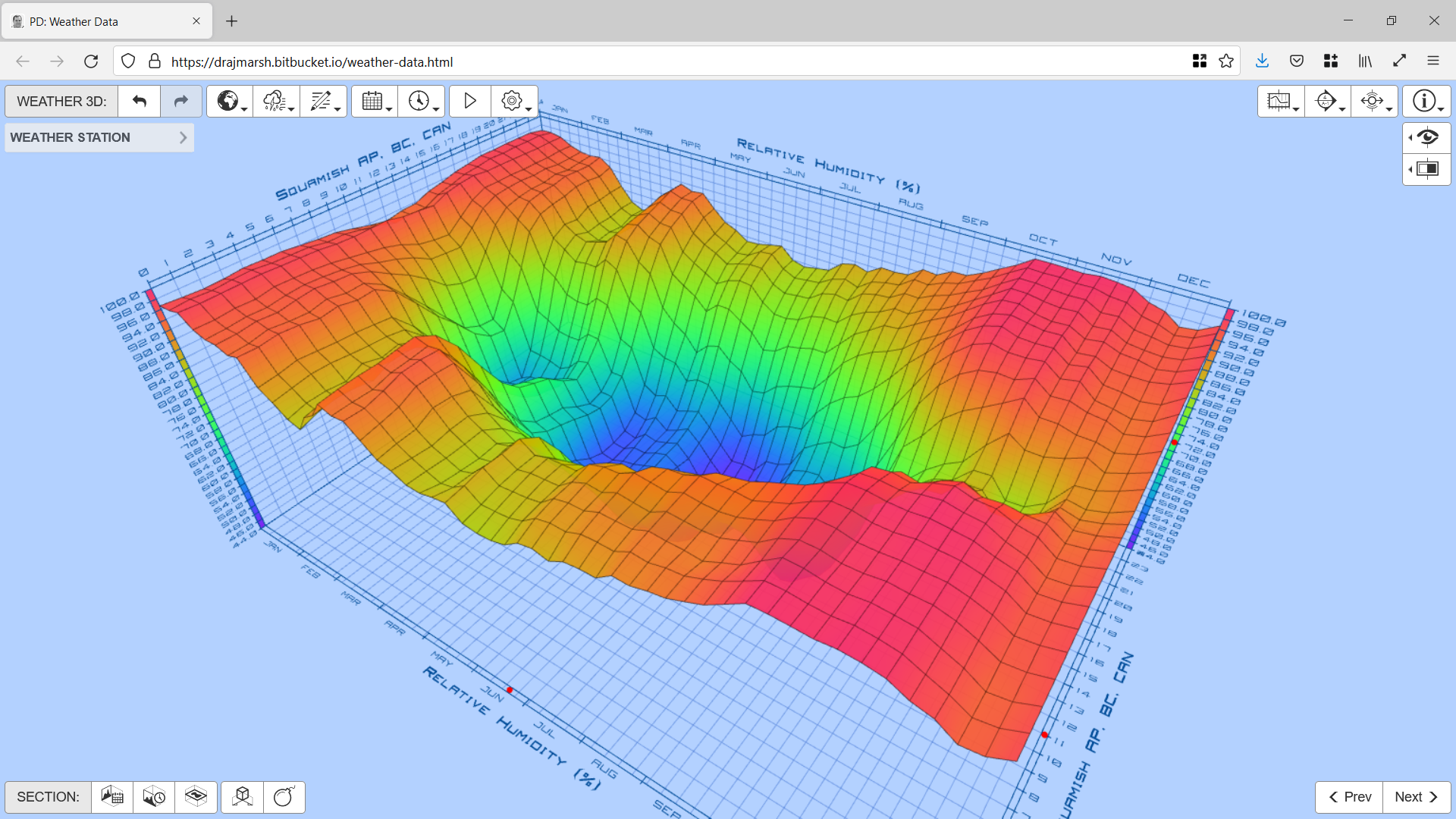
Figure 13 Andrewmarsh.com; Weather Data Viewer
Climate Consultant Software
Climate Consultant is another simple to use, graphic-based computer program that helps architects, builders, contractor, homeowners, and students understand their local climate. Most climate elements available in an EPW file can be translated to a quick to understand diagram. The drawback of this software is that saving images is not possible. The only way to get around is to use screenshots, that make it hard to get high quality imagery.
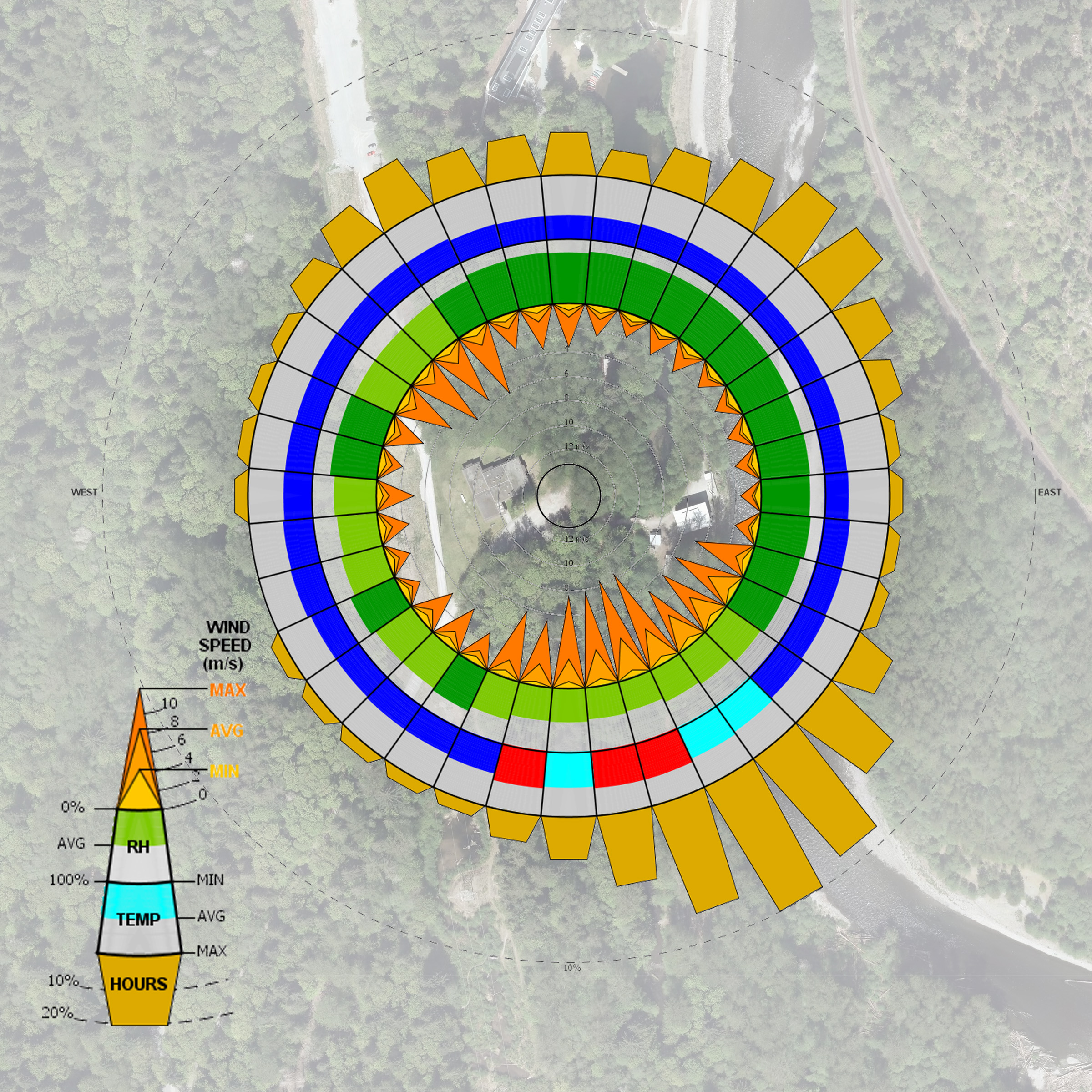
Figure 14 Windrose Diagram from Climate Consultant Superimposed on Site Aerial
Psychrometric Chart
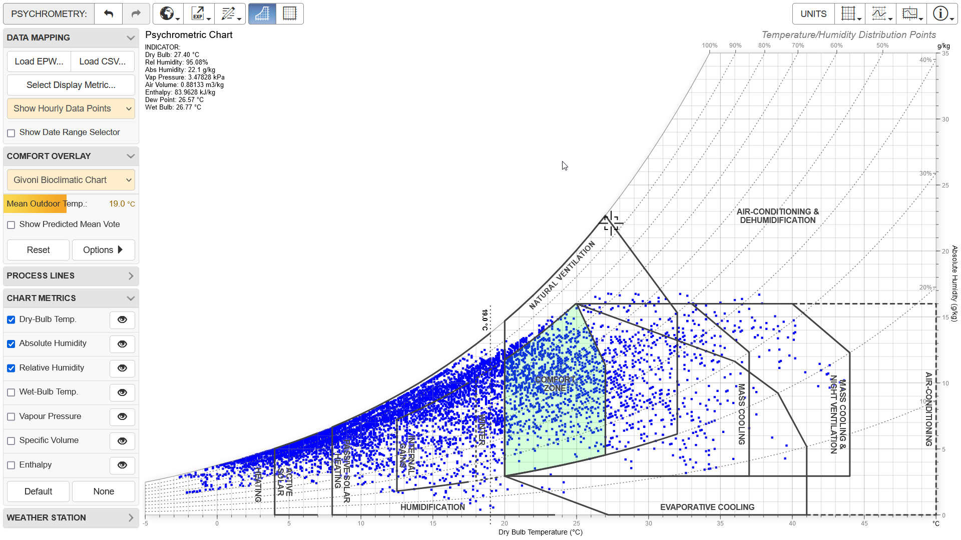
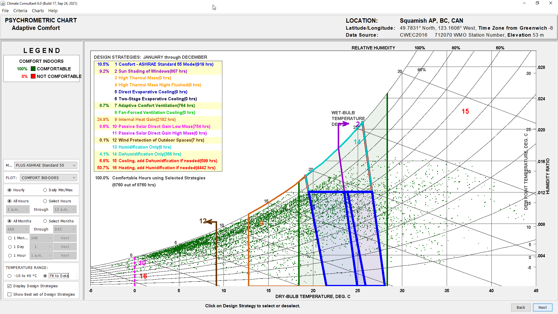
Both Climate Consultant as well as Andrew Marsh offer a psychrometric chart tool that overlays the EPW climate data with comfort metrics. A psychrometric chart is a graph that allows to study moist air and its thermodynamic parameters (at assumed constant pressure). All 8760 data points for each hour of the year can be plotted individually or shown clustered in a density grid with heat map overlay. The thermodynamic relationships between air temperature and moisture are key factors in determining human comfort and are therefore an important part in climate responsive and/ or passive design. Understanding psychrometric charts can help you visualize environmental control concepts, such as why warm air can hold more moisture or, conversely, how allowing moist air to cool will lead to condensation. Most psychrometric charting tools allow you to overlay either comfort definitions based on various standards (e.g., ASHRAE 55, EN 15251) or even suggested passive or active design strategies (based on assumptions about building type and performance level).
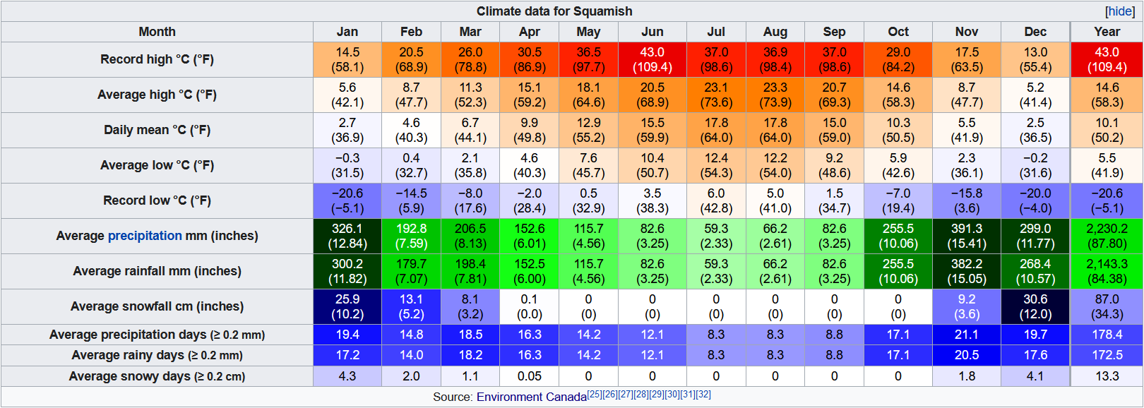
Precipitation Data
Even though the EPW format reserves data columns for various kinds of precipitation data it is typically not present in those weather files available in the public domain. To find out about average precipitation, rainfall, snowfall, and snow depth Wikipedia, weatherbase.com or weatherstats.ca is usually a good source to go to. As the amount of this monthly data is still somewhat easy to juggle you could revert to Microsoft Excel to translate to desired diagrams.
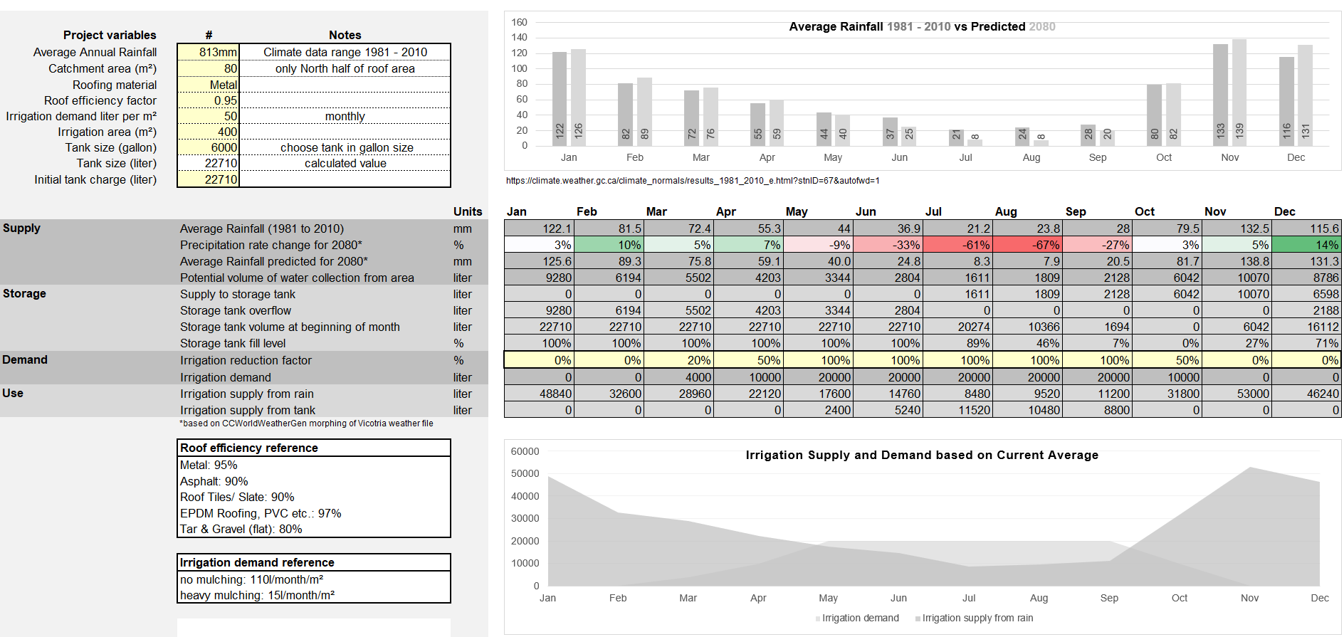
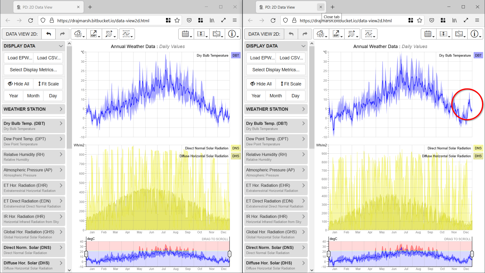
Comparing Weather Files
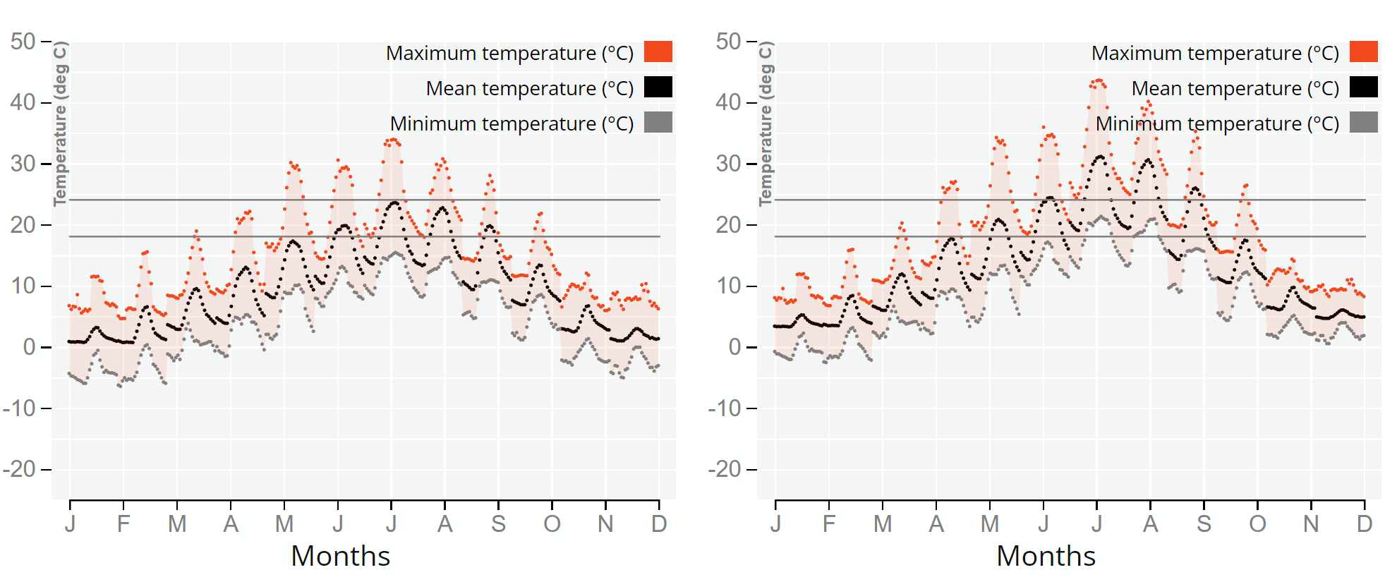
If you want to visually compare two different locations using the andrewmarsh.com tools, you will have to open two browser window side by side and set the scale minimum and maximum to the same values for both locations. This can be a useful tool to scrutinize multiple datasets for the same location and find oddities or inconsistencies. The example below shows two files that are available via building.one.org for the Squamish airport location. On the left is *CWEC2016.epw and on the right the *TMYx.2004-2018.epw file.
Probably the most feasible use case to compare weather files is to explore patterns of climate change between a measured datasets and a datasets that has been morphed into the future (e.g., the year 2100) to simulate future climate conditions.
Methods for assessing future climate conditions for building design
Resiliency of buildings to climate change is becoming more and more part of design briefs. So far, the resiliency strategies have been addressed qualitative and anecdotally. Recent ability to morph climate data into the future by “superimposing” IPPC climate models on local measured data and the publication of those files in EPW format by commercial entities, academia or governments make it possible to quantify impacts for example on cooling loads or examine feasibility of passive measures. Future morphed climate data is not standardized but will always be based on locally measured TMY data with a version of IPCC assessment model overlay to transform the measured data. Data projections of the future climate are inherently uncertain and will only estimate a likely range.
Shifting Weather Files into the Future
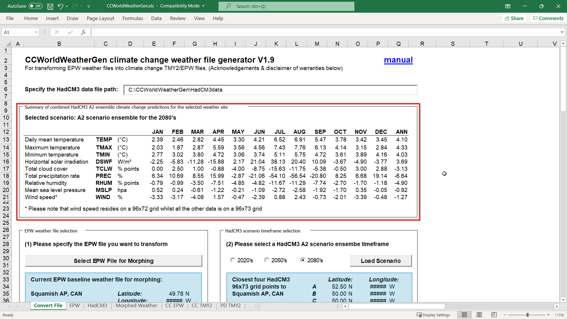
- A DIY approach is available through the University of Southampton. They have published a tool based on Microsoft Excel that loads local EPWs and “mashes” this data with assumptions based on the IPCC Third Assessment Report. The tool is called Climate Change World Weather File Generator for World-Wide Weather Data – abbreviates as CCWorldWeatherGen[6].
- The WeatherShift project, a collaboration between Arup and Argos Analytics allows to “shift” any available EPW in three steps into the years 2035, 2065, and 2090. A selection of graphical that represent
- The proprietary software Meteonorm[7] by the Swiss based Meteotest AG can generate future simulation weather data in 10-year steps based on the IPCC RCP scenarios (RCP 2.6, RCP 4.5, RCP 8.5) up to the year 2100. Beyond the EPW format this software can export 30+ formats for building and renewable energy simulation packages.
- The BC based Pacific Climate Impact Consortium recently published future shifted climate data sets
Climate Change-Modified Weather Files in Energy Modeling
All multi-zone dynamic energy modelling (operational energy simulation) software packages that can read EPW weather files can also be used to simulate building performance according to future conditions. Below are some tools that are used in architectural design practice:
- Sefaira
- WUFI
- cove.tool
- Rhino & Ladybug/Honeybee
- ClimateStudio
- Design Builder
- Openstudio
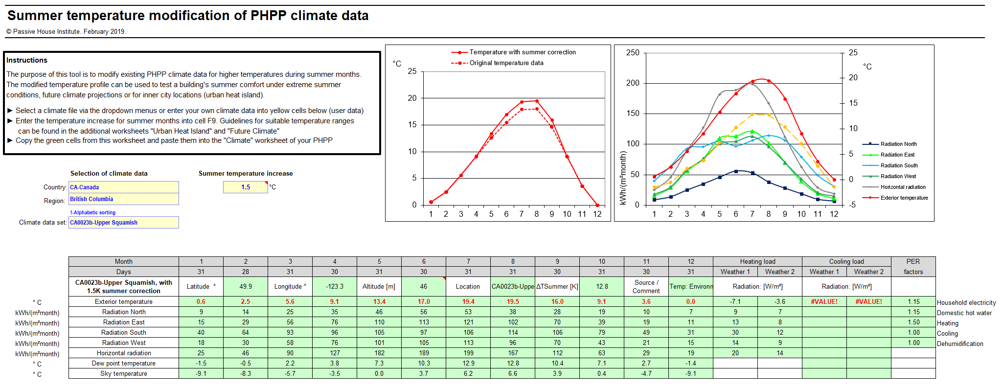
The Passive House Planning Package (PHPP) can be used with the Summer Temperature Tool provided by PHI[8] to create a custom climate file to do stress testing on overheating and cooling for either future summer conditions or urban heat island effect. The above mentioned Meteonorm also allows to export PHPP compatible historic or future shifted climate data. Beware that for certification you should always confirm that the climate data set you are using for Passive House modeling is approved by PHI.
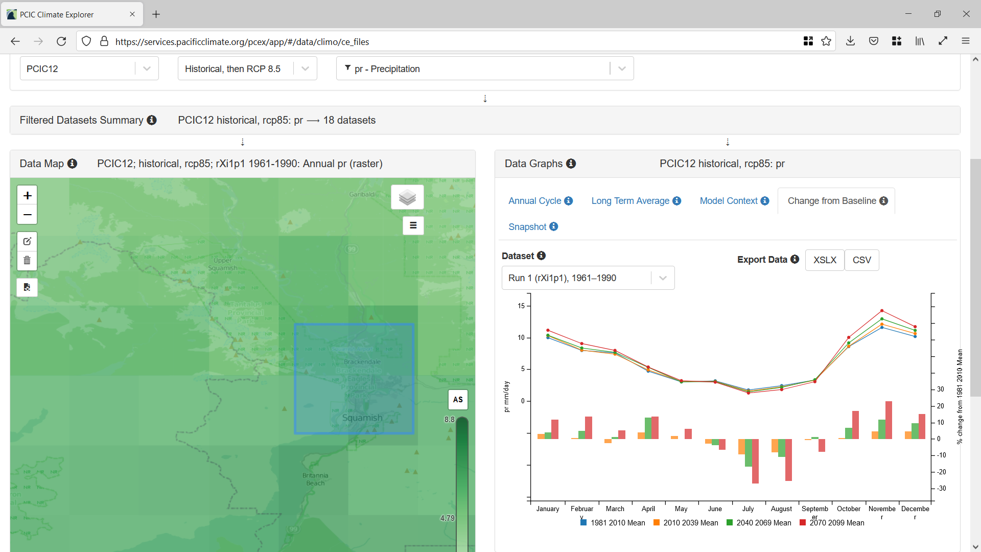
Climate Atlas of Canada
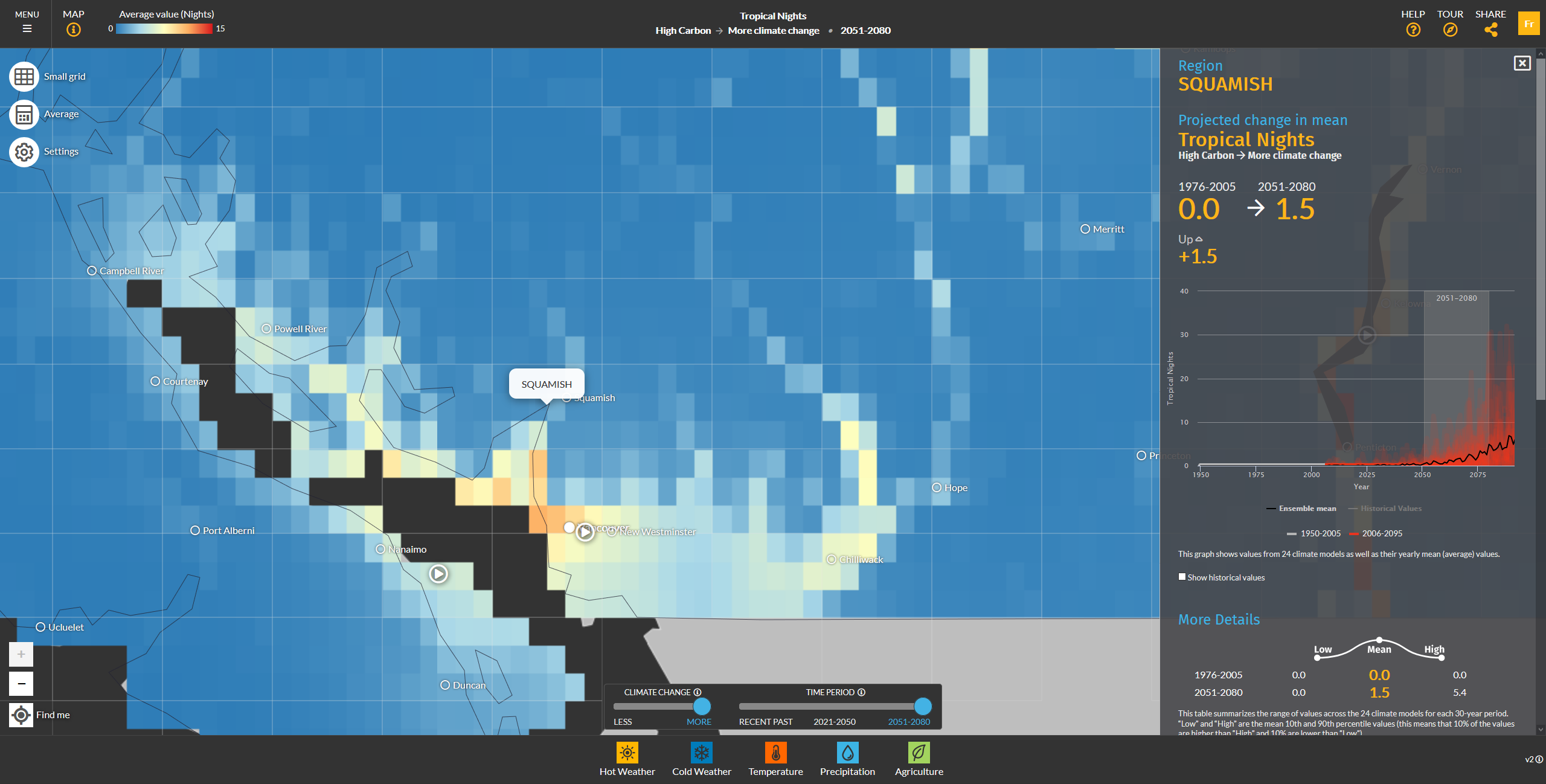
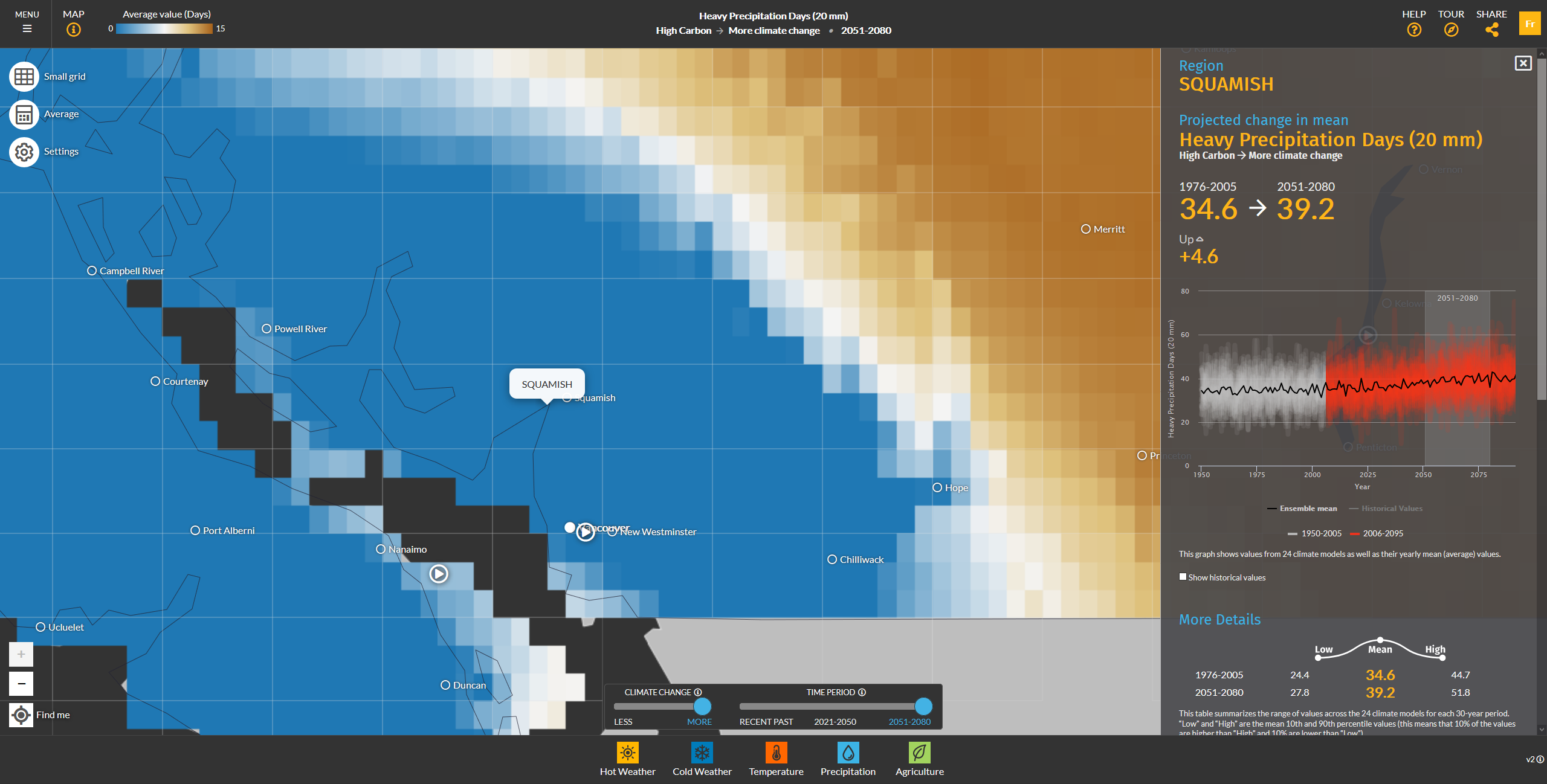
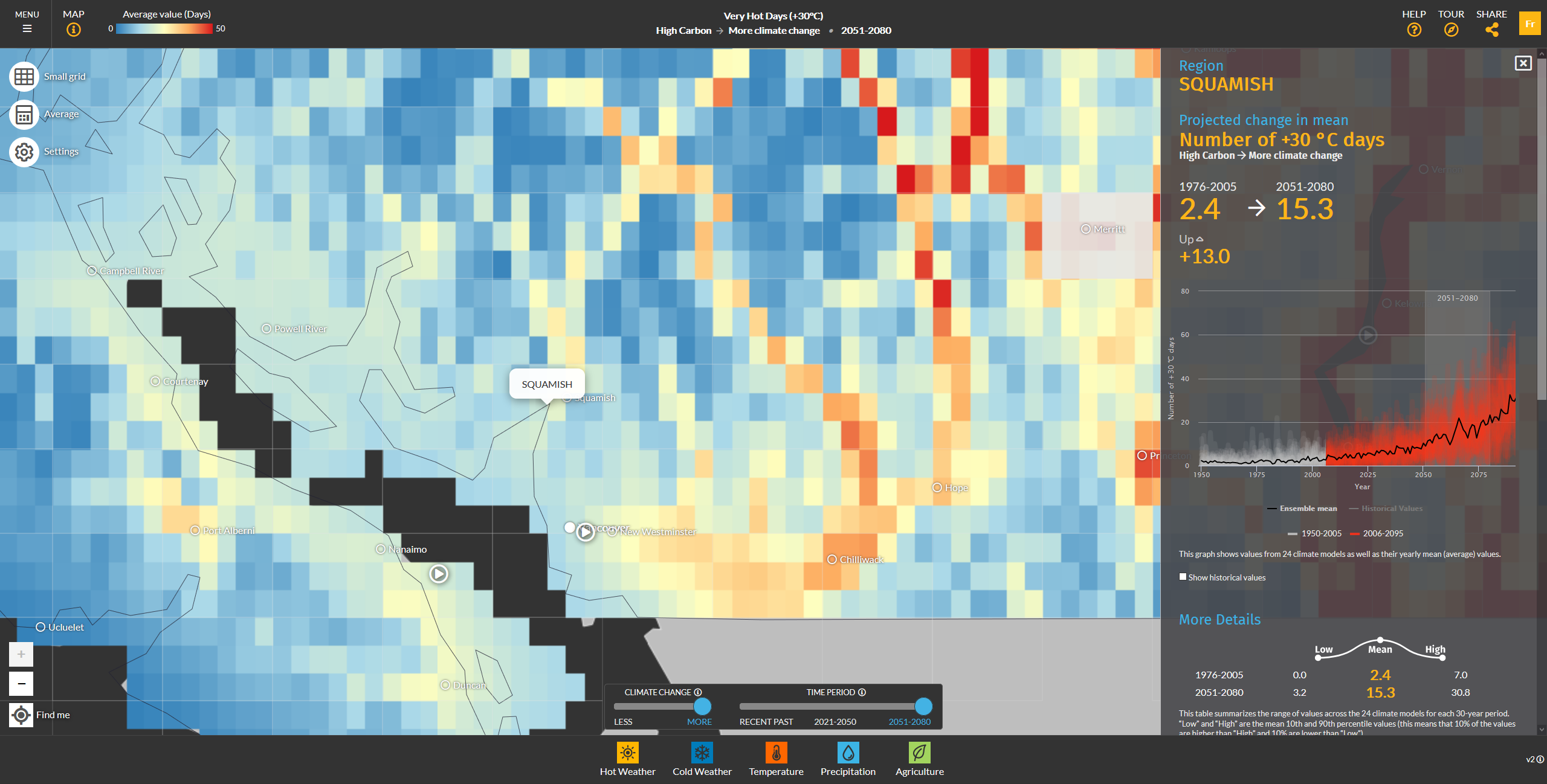
The Climate Atlas of Canada was created by the Prairie Climate Centre at the University of Winnipeg. It is an innovative climate science and communications tool that allows users to visualize and interact with climate data as well as the human stories about climate change and climate action on the landscape from coast to coast to coast.[1]
The Climate Atlas is a communication and mapping tool that is built on 24 global climate models that shows average projected changes up to 2080 into the future compared to the 1976 – 2005 baseline for major climate metrics. The mapping tool covers all of Canada, in the South a grid resolutions of the data is as fine as ca. 60km x 30km grid cells. You can download summary reports (PDF), climate model data and historical data (tabular, CSV) as well as graph images for each particular region (grid cell). The information is geared to decision makers to help assess climate risks for building and infrastructure design, agriculture etc.
Climate Classification Mapping
The Köppen-Geiger system classifies climate into five main classes and 30 sub-types. The classification is based on threshold values and seasonality of monthly air temperature and precipitation. According to this classification system representing today’s conditions the Cheakamus site lies at the border of the Dfb region (Humid Continental Mild Summer, Wet All Year) to the Cfb region (Temperate Oceanic Climate).
This visualization can be best appreciated when animated.
Add H5P sliding image
ArcGIS StoryMap website[9] or download climate shifts overlays (KML format) for Google Earth to interactively explore the changing climate zones[10].
Specific Site Analysis based on GIS Data
In this chapter we want to discover the possibilities of combining GIS data either from widely available public sources or collected specifically for the project via drone or photogrammetry.
Automated Creation of Digital Terrain Models (DTM) from GIS Data
Any landscape or site is a whole system, yet one composed of elements or parts, in the early predesign phase you should analyse them. One of the first things that define the ecological context is the surface of the earth that acts as the inface of lithosphere and atmosphere. The intent is to show how we can utilize various data interfaces and software applications to bring environmental data into our digital architectural design hub (with a focus on common software in our market like Revit and Sketchup). Some of the following briefly described methods based on specialized plugins and scripts have the benefit of ease of use but are constrained in other ways. The table shown below the listing tries to illustrate those benefits and drawbacks. If none of the listed software either does not give you the satisfactory level of detail and you have access to GIS information for example via a municipal open data portal, you can go the hard and manual route converting this available open data using the open-source GIS system QGIS to create a site context model for use in Revit or Sketchup.
Placemaker for Revit
https://www.suplacemaker.com/
High resolution terrain data, roads, building masses, even existing trees right in Revit. Expensive subscription required.
Revit & Dynamo with the GIS2BIM Dynamo Package
https://github.com/DutchSailor/GIS2BIM
Connects to WMS (Web Map Services), ARCGIS Map Services, Google API, GEOTIFF, etc. Slow interface. You have the data right in Revit.
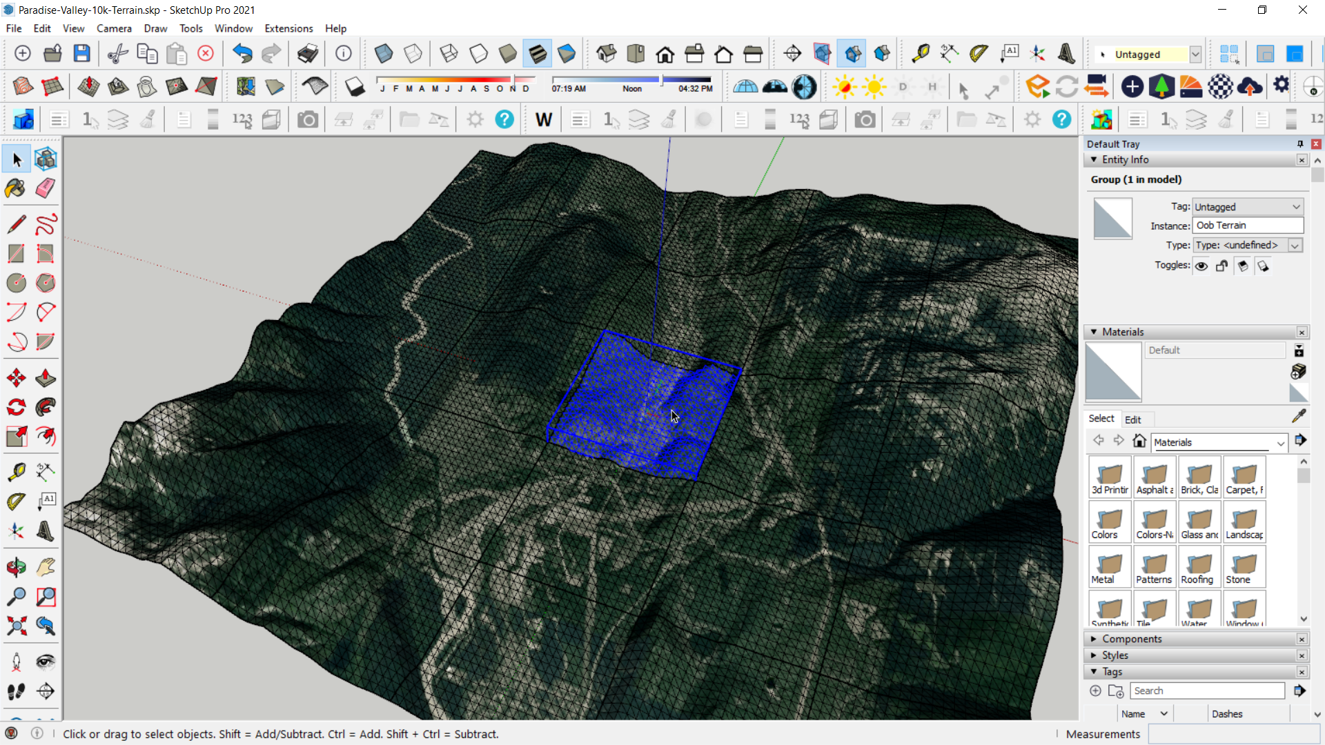
SketchUp with the Oob terrain plugin
http://oob.duckdns.org/terrain/
Terrain, building massing, satellite or map textures, no trees.
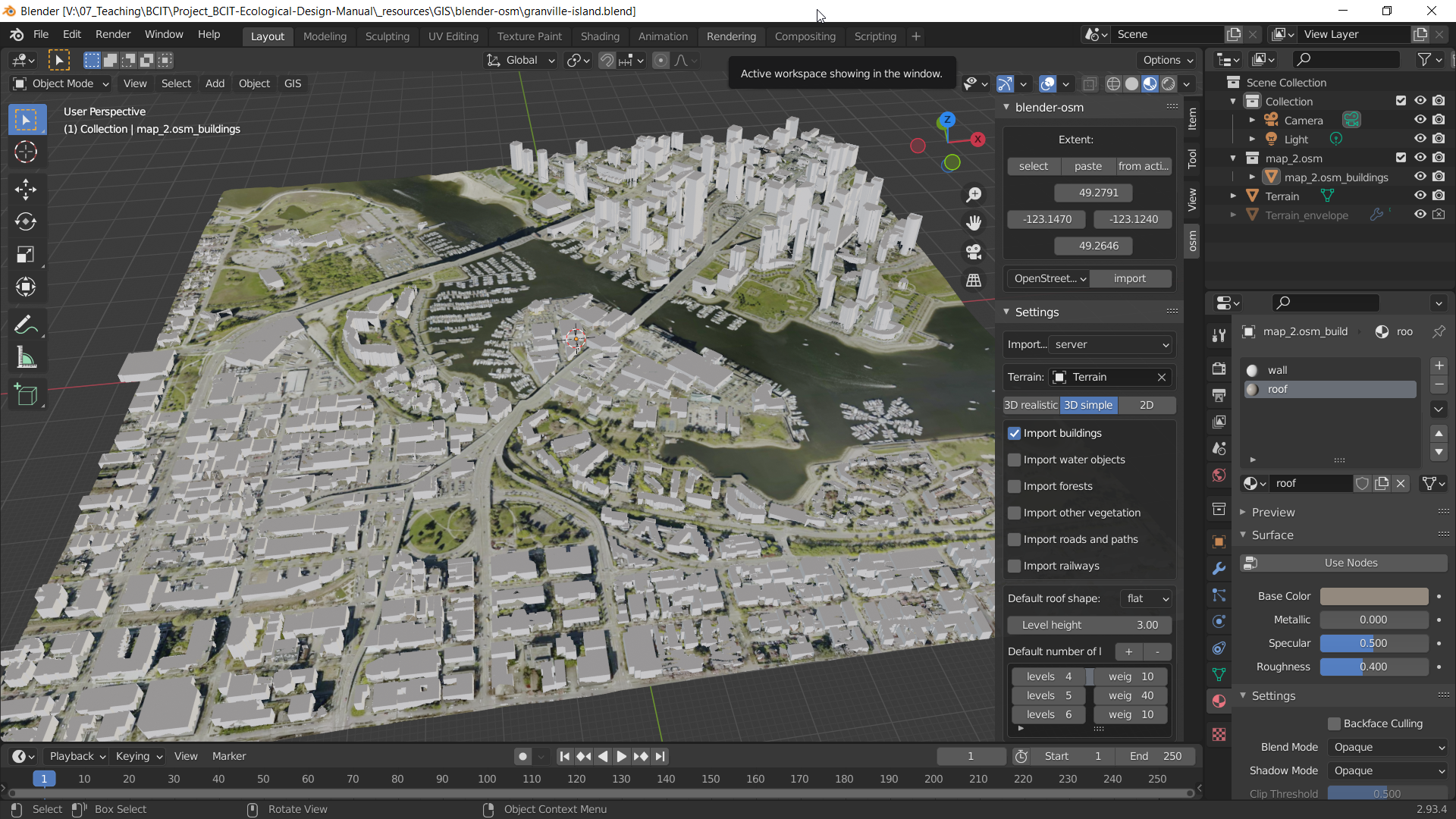
Blender with the blender-osm or blender-osm premium addon
https://prochitecture.gumroad.com/l/blender-osm
Terrain, building massing, satellite and map texture, trees. Conversion from blender to typical design environment might be more difficult.
Blender with the BlenderGIS addon
https://github.com/domlysz/BlenderGIS
Free and open source, access to many common GIS file formats within a 3D modeling environment like Shapefile vector, raster image, geotiff DEM, OpenStreetMap xml). Conversion from blender to typical design environment (Revit, Sketchup) might be more difficult.
Manually Convert Open Data with QGIS to a Revit Toposurface
There a great benefits to creating and managing the site context for your building right in Revit as opposed to import surface polygon geometry from other programs. If you are using the native massing and site tools (create a toposurface via a 3D terrain contour drawing or point file) you will get the benefit of being able to easily manipulate geometry and control the visibility of objects. For example you can do cut-and-fill calculations, edit the topography localized, and create building pads or excavation. You can also conveniently place trees and other site objects on the topography. More detail and context can be shown by using a high resolution aerial image texture on the site material. QGIS is a great and free software to produce the necessary input (3D contours, point cloud) for further processing in Revit.
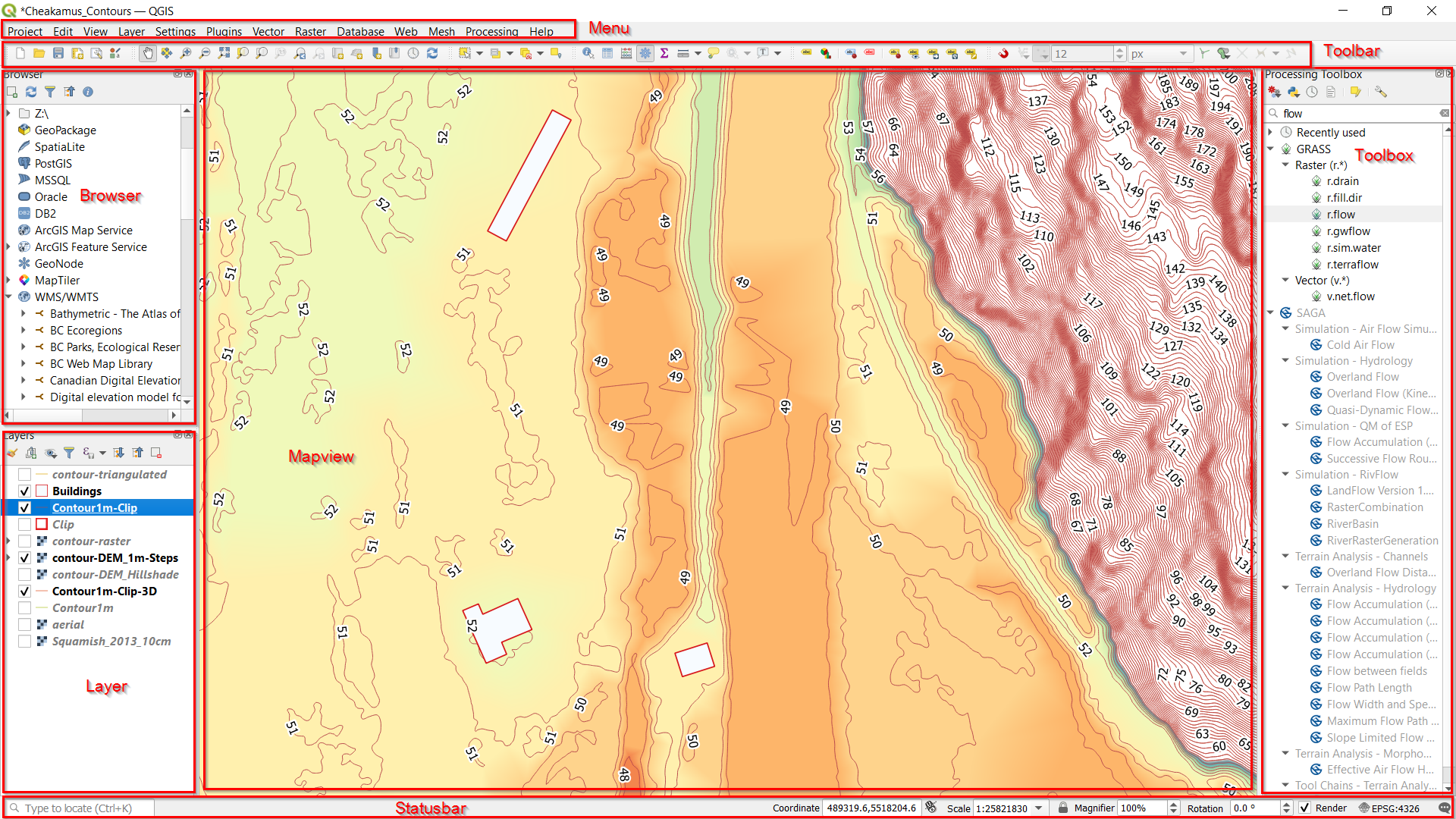
The steps below show how the highly detailed contour data set provided by the municipality of Squamish (https://data.squamish.ca/datasets/contour-1meter/) can be converted to serve as useful context in the Revit design environment. The result might be a too “heavy” geometry to navigate in Revit. To maintain swiftness and fun continuing with the building design you should find a balance between the size of your area of interest, the level of detail of your terrain and size of the geometry created. Architectural software generally will struggle more with data size then dedicated GIS tools.
- Download and install the latest version of QGIS from https://qgis.org/en/site/
- Download the Shapefile version of the “Contour 1 meter” at https://data.squamish.ca/datasets/contour-1meter/explore
- Download a georeferenced aerial image (TIF or EPW format) that covers your area at https://data.squamish.ca/search?appid=4c582f55cfd8479cb27f39b87af817ef&collection=App%2CMap&edit=true&type=image%20service
- Create a new project within QGIS and drag the Shapefile (SHX or SHP) and the aerial image file (EPW or TIF) into the map view of the program. Because both files are georeferenced, they should position exactly aligned without edits.
- Save your file into a dedicated project folder.
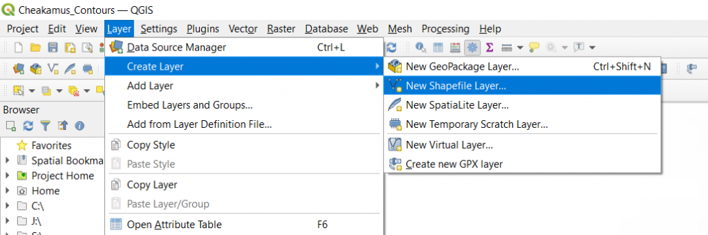
- Create a new layer via the menu item Layer/Create Layer/New Shapefile Layer…
- Right click this layer in the layer manager and choose Toggle Editing from the context menu.
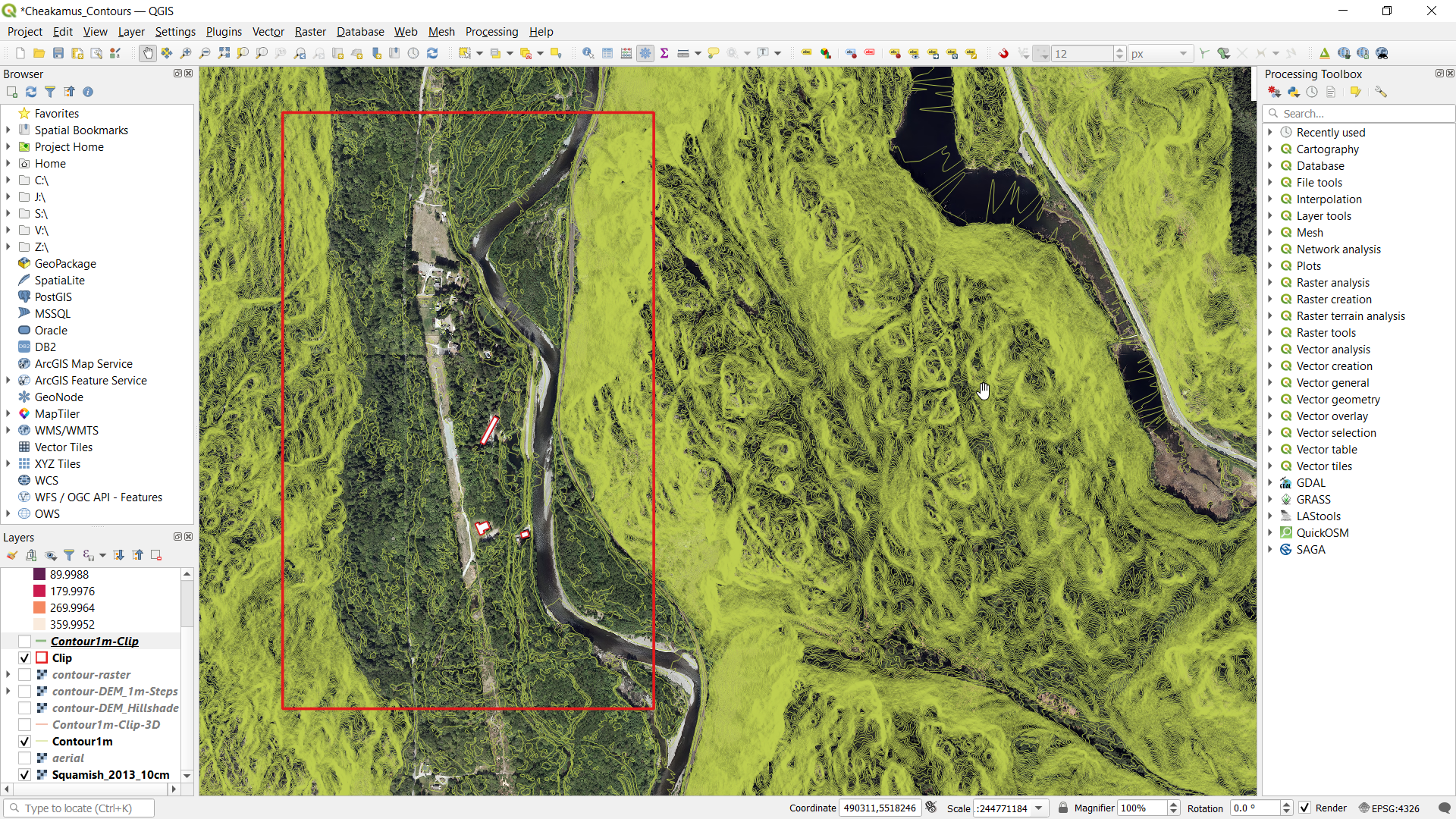
- Draw a rectangle that represents your scope area. This rectangle will be used to clip the excess data before you export into the architectural software.
- Right click the layer again and choose Properties…
- Under Symbology set the appearance to “outline red”
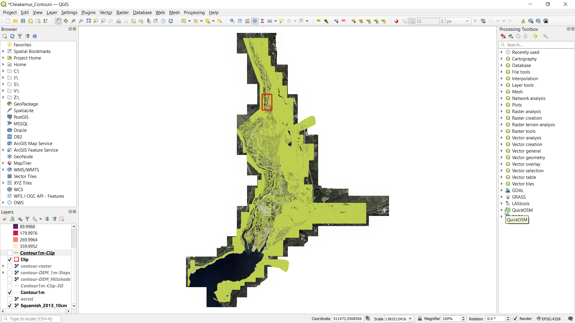
- Go to the View menu item and under Panels check the Processing Toolbox item on. This panel should appear to the right or your map view.
- Type “clip” into the search box. This will bring up various commands to clip raster and vector layer.
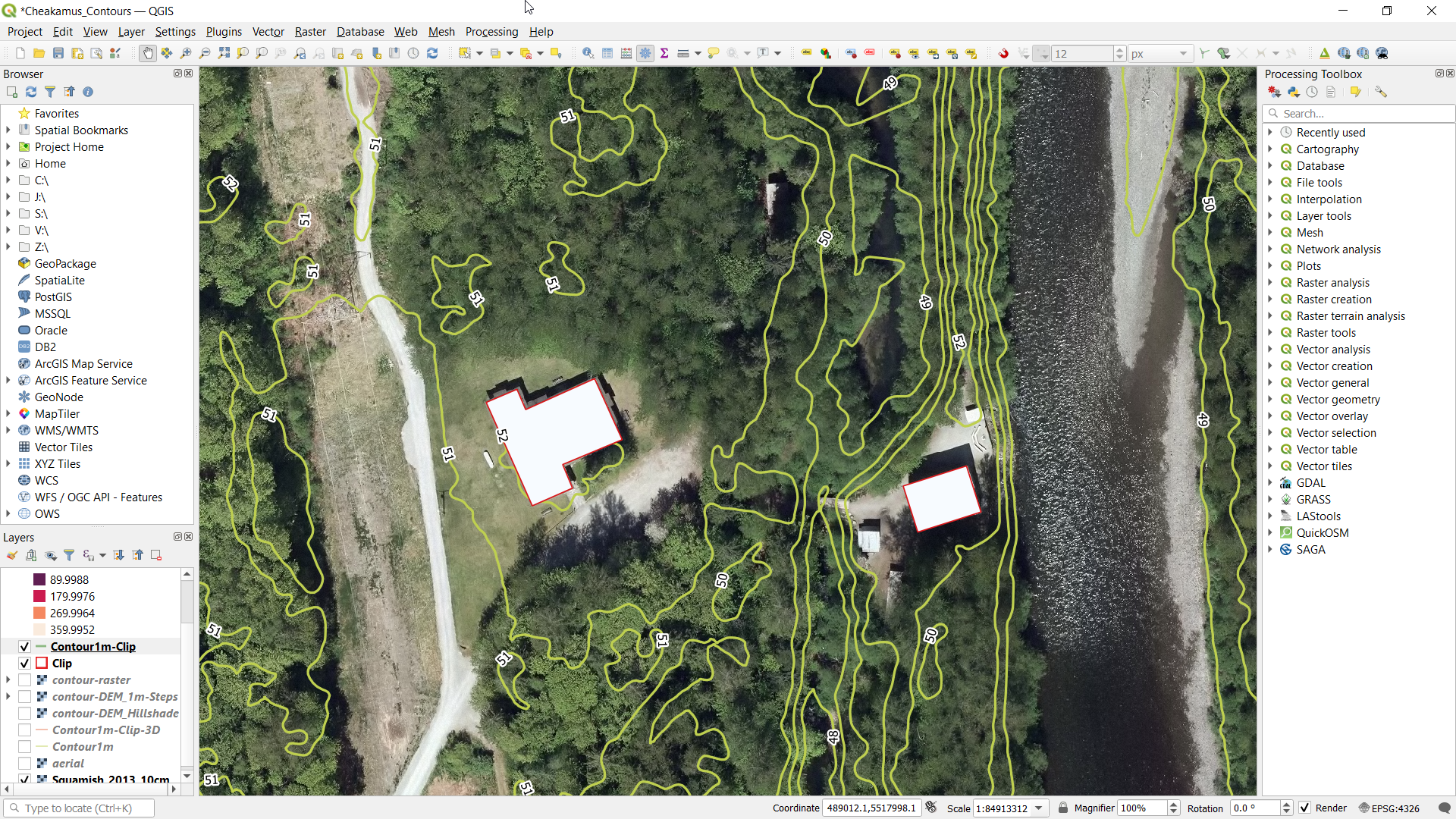
- Use the Clip raster by mask layer on the “Squamish_2013_10cm” aerial image layer and save the resulting layer as a TIF file. The benefit of TIF is that it is still georeferenced as well can be opened in Photoshop for editing later.
- Use the Clip vector by mask layer on the “Contour1” layer and save the resulting layer at the same time as a Shape layer.
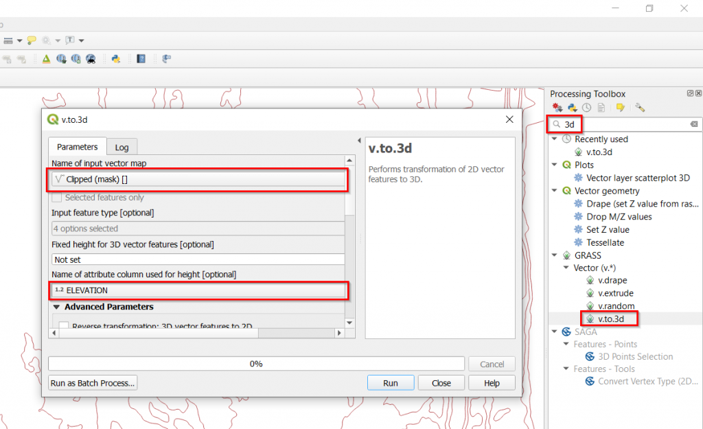
- Type “3d” into the search box of the Processing Toolbox. Under GRASS your should find a command called v.to.3D.
- Use the v.to.3D command on the clipped vector layer representing the contours. Make sure that you use the attribute that represents the elevation (in our case ELEVATION or ELEV) to set the height of the linework. After you used this command, you have a new layer that now consists of 3D polylines ready to be exported into a 3D DXF file.
- Right click this new layer and choose Export/ Save this Feature as… Choose DXF as the format and make sure the Include z-dimension is checked
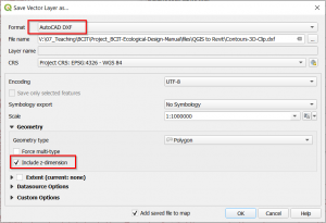
- Open the file and save as a DWG format.
- In Revit link this DWG (pay attention to scaling, uncheck Correct lines and Orient to View)
- Create a Toposurface by choosing the linked DWG.
- Create a new material that is textured with a JPG copy of the clipped aerial image from the QGIS process (the texture needs to mirrored and rotated 90 CW in photoshop and the texture dimensions need to equal the dimensions of your toposurface).
- Now you can go ahead and set your base elevations, and model your context infrastructure etc.
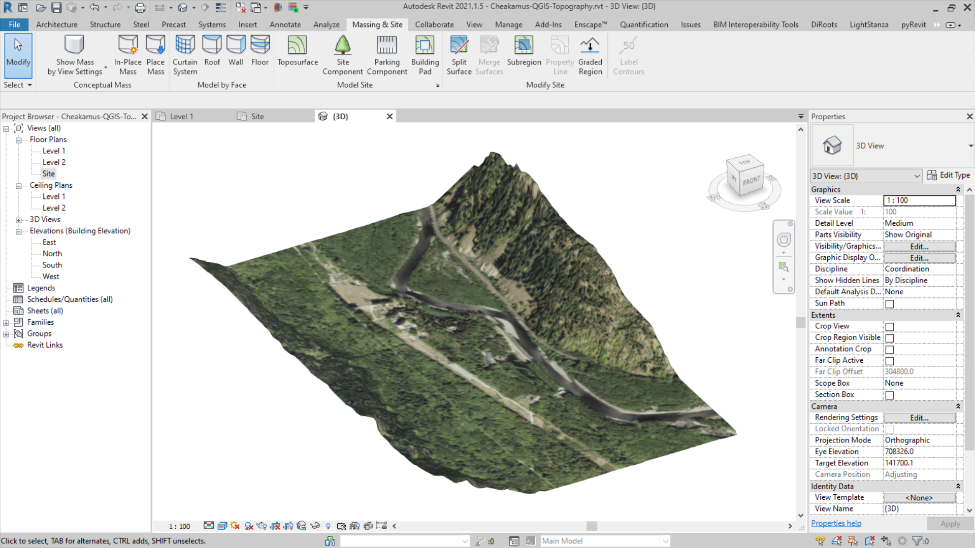
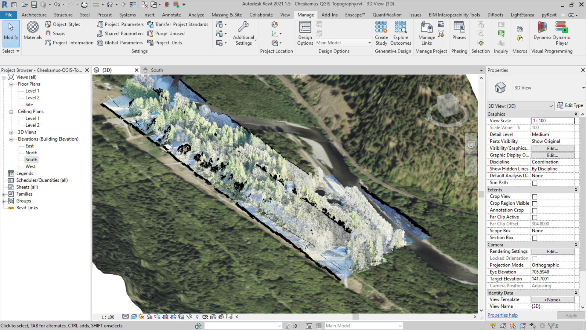
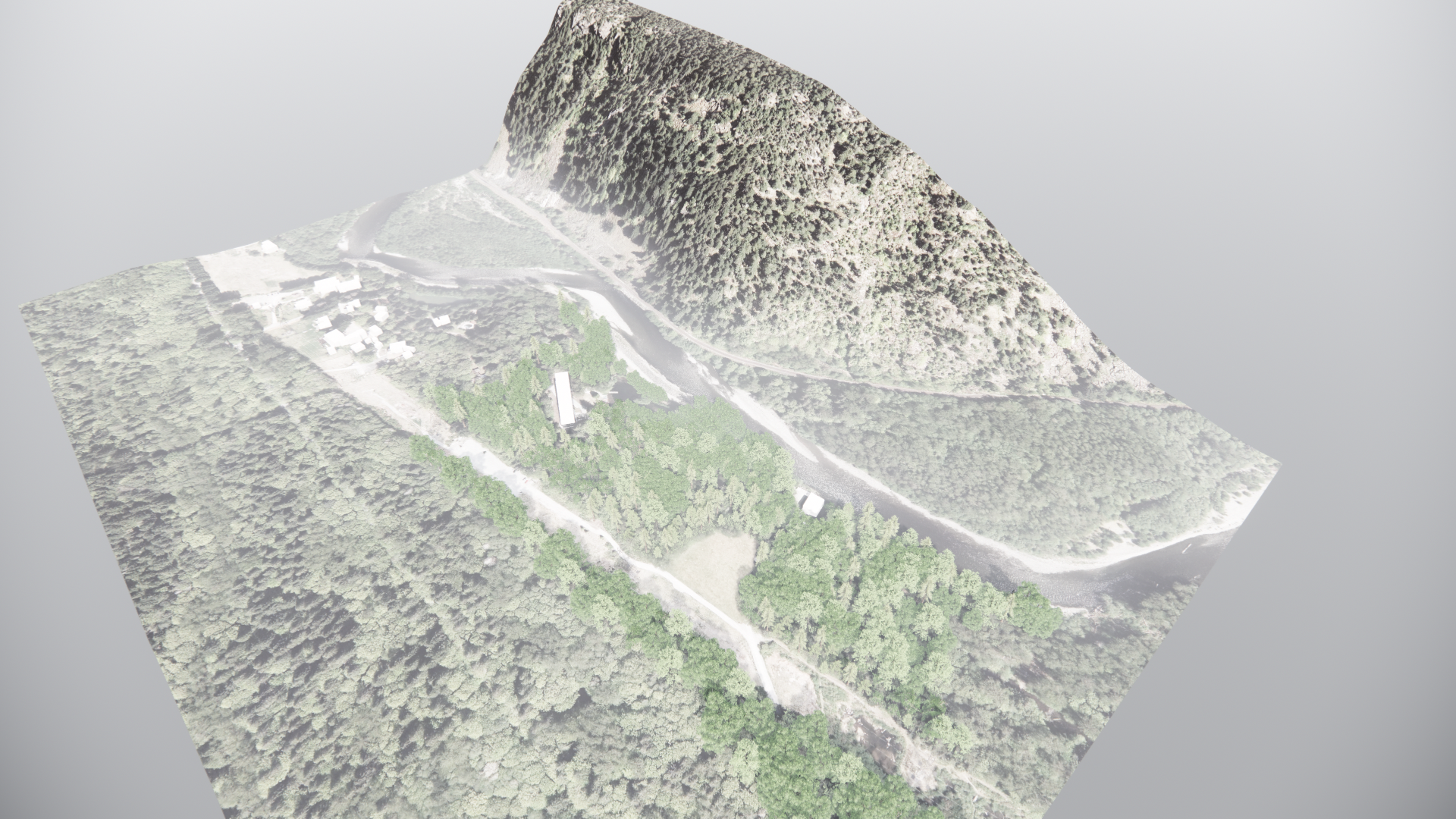
The site context model below is created in Revit with imported contour data from the Squamish Open Data Portal, tree models were placed manually based on the 3D point cloud envelope, and visualized with Enscape. The tree type mix was approximated based on site observations and literature. This is a fully flexible native Revit Toposurface that allows you to locally edit the topography and create building pads to place design intent models.
Selected Geospatial Data Sources
- BC Geographic Data (https://www2.gov.bc.ca/gov/content/data/geographic-data-services)
- iMapBC (https://www2.gov.bc.ca/gov/content/data/geographic-data-services/web-based-mapping/imapbc, this site allows to view and download layers and GeoTIF)
- DataBC (https://catalogue.data.gov.bc.ca/dataset?download_audience=Public)
- LidarBC (https://www2.gov.bc.ca/gov/content/data/geographic-data-services/lidarbc)
- Metrovancouver Open Data Cataloge (http://www.metrovancouver.org/data)
- Squamish Open Data (https://squamish.ca/discover-squamish/maps-and-data/open-data/)
- City of Vancouver Open Data Portal (https://opendata.vancouver.ca/pages/home/)
- Burnaby Maps & Open Data (https://www.burnaby.ca/services-and-payments/maps-and-open-data)
- City of Surrey Open Data (https://www.surrey.ca/services-payments/online-services/open-data)
- CRD Open Data (https://www.crd.bc.ca/about/data)
- District of the Fraser Valley Mapping (https://www.fvrd.ca/EN/main/services/mapping.html)
- Township of Langley Open Data (https://data-tol.opendata.arcgis.com/)
- New Westminster Open Data (http://opendata.newwestcity.ca/)
- District of North Vancouver Open Data (http://www.geoweb.dnv.org/data/)
- District of West Vancouver Open Data Portal (https://mapping.westvancouver.ca/OD/dbo_OPENDATA_FILES_list.php?page=list)
- Island Trust Mapping (https://islandstrust.bc.ca/mapping-resources/mapping)
- CADMAPPER (contour files with 4m increments, based on the OpenStreetMap collaborative, https://cadmapper.com/)
Create a Panorama Sun-Path from a Digital Terrain Model
For low-energy passive architecture and solar renewable energy use (photovoltaics, solar hot water), knowledge about the availably of the precious solar resource is key for success. Knowing when overshadowing from neighbouring hills, buildings or trees help to lower cooling loads will help to passively keep the building cool in summer. If you are working on an urban design scheme you even have control over the solar envelope for each parcel/ building block[11].
To assess the solar azimuth angle and zenith angle for key times of the year various 2D and 3D solar path diagrams can be used. 3D solar path diagrams can be integrated with building, context, tree, and topography geometry to learn about potential overshadowing.
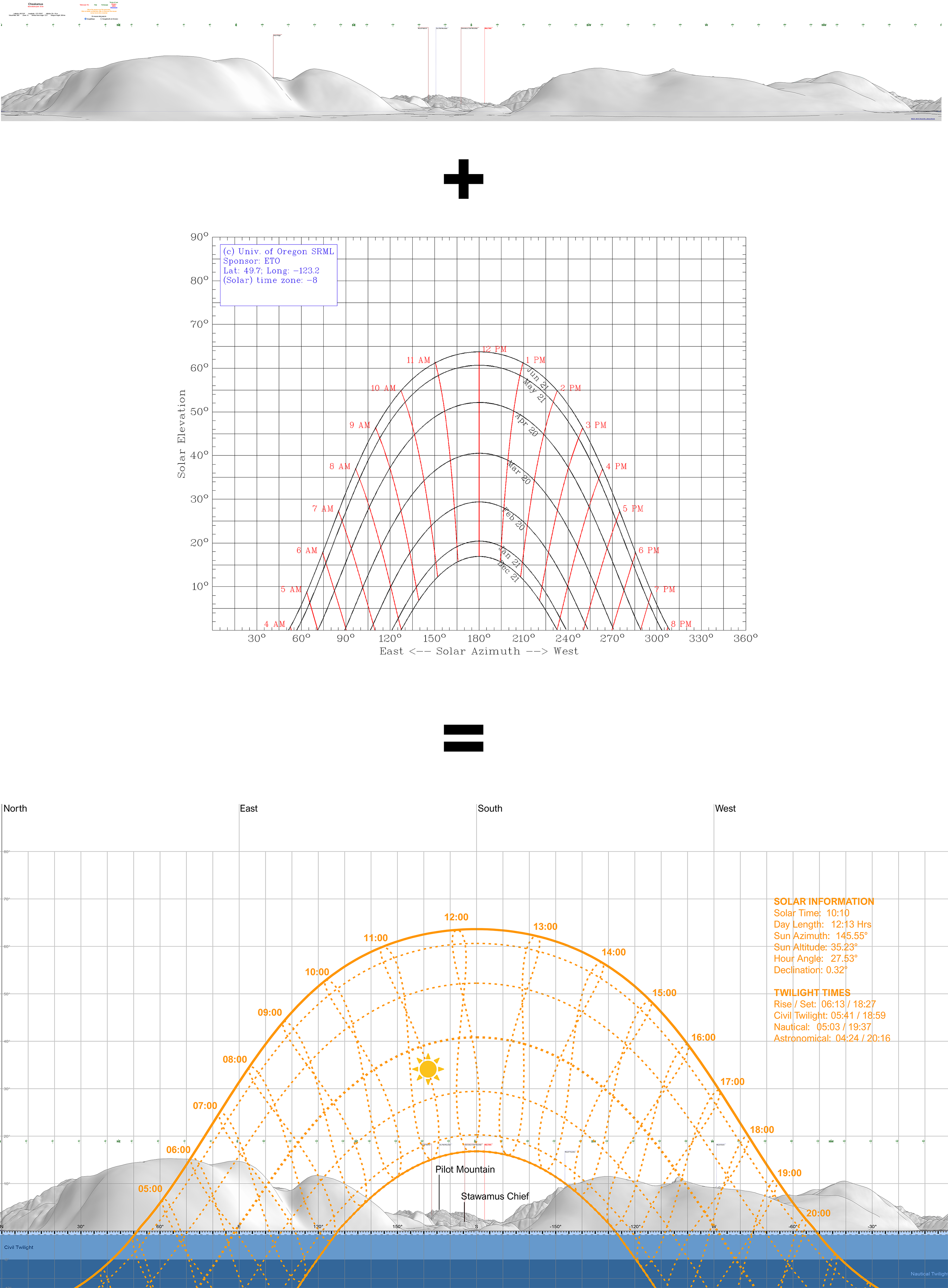
If we are designing in a rural transect, or a mountainous region where the topography might be a considerable shading factor we can use a panoramic sunpath overlay to assess the shading of hills and mountains over the course of the year. A DEM based panorama can be generated through this website: https://www.udeuschle.de/panoramas/makepanoramas_en.htm. This site uses NASA Shuttle Radar Topography Mission data and other open-source databases for the digital elevation model as well as geographical names.
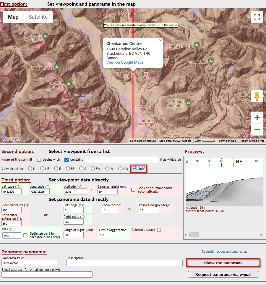
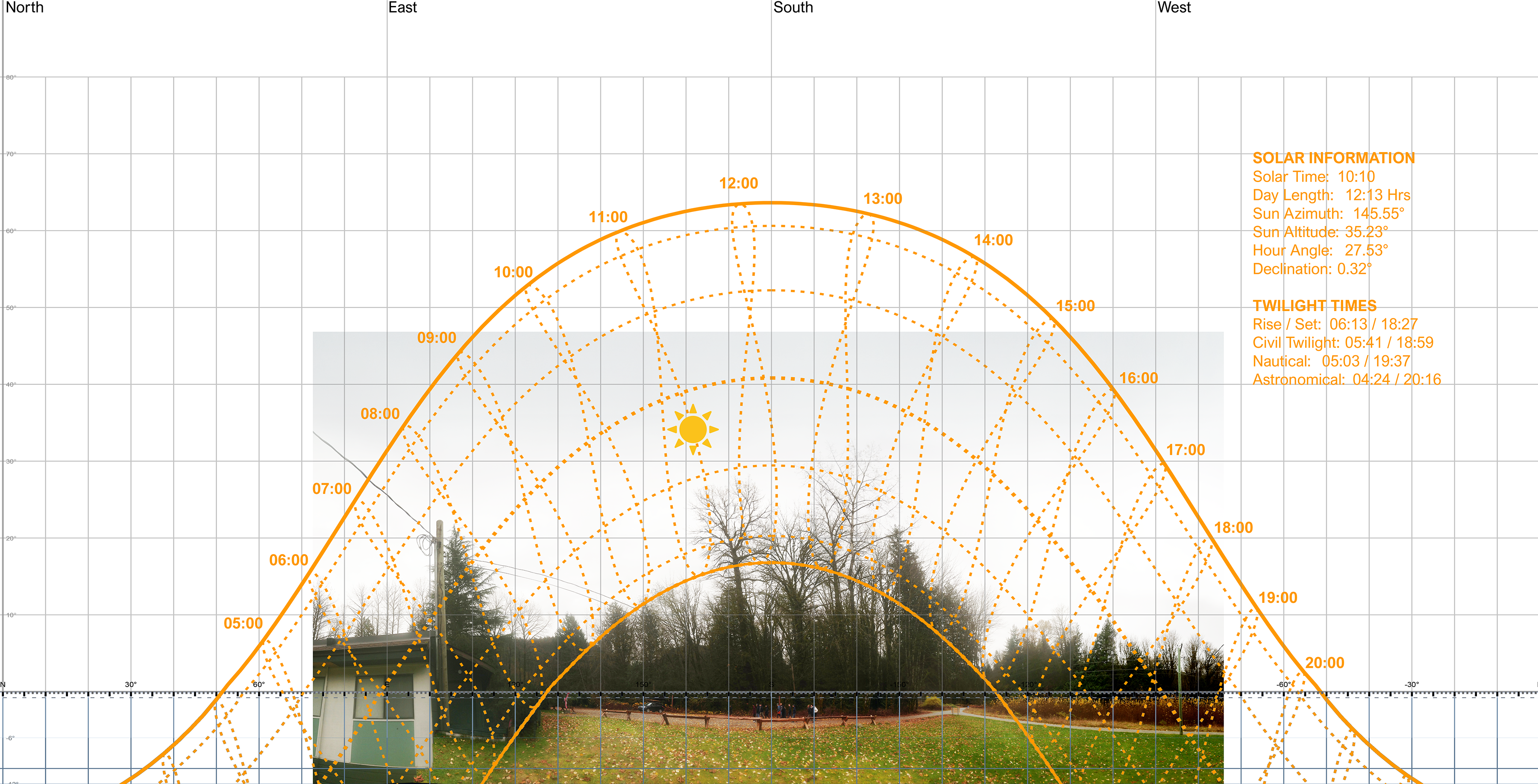
After choosing your site and height above ground in the udeuschle.de web app, then check to create a 360º panorama in the view direction setting, then download the panorama image via the Show the panorama button. A high-resolution panorama tiled image will pop-up in a new window. You will have to use the browser integrated screenshot function to download. By triangulating one of the known peaks on the panorama you can calculate the inclination angle. This information, and the noted cardinal directions will give you the anchor points to superimpose a cartesian sun-path diagram in a graphic editor (like Adobe Illustrator). The sun-path diagram for this instance was generated at andrewmarsh.com 2D Sun-Path web app and downloaded as a SVG (scalable vector graphic).
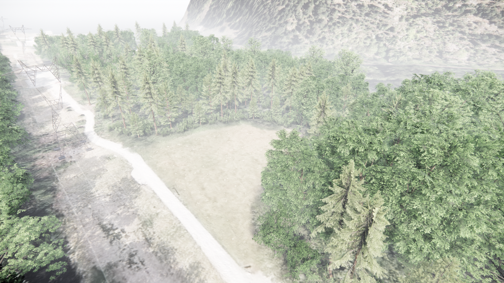
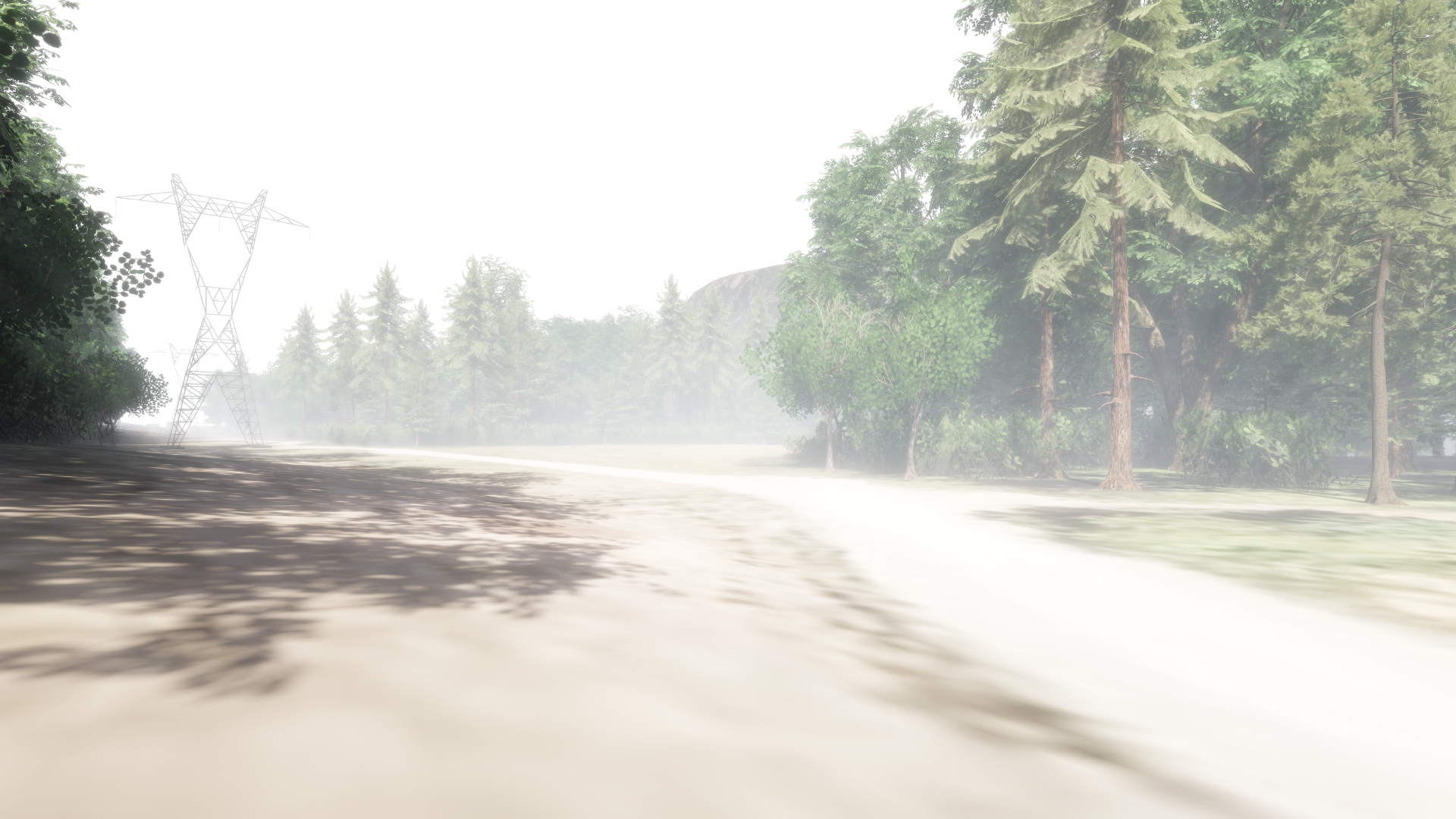
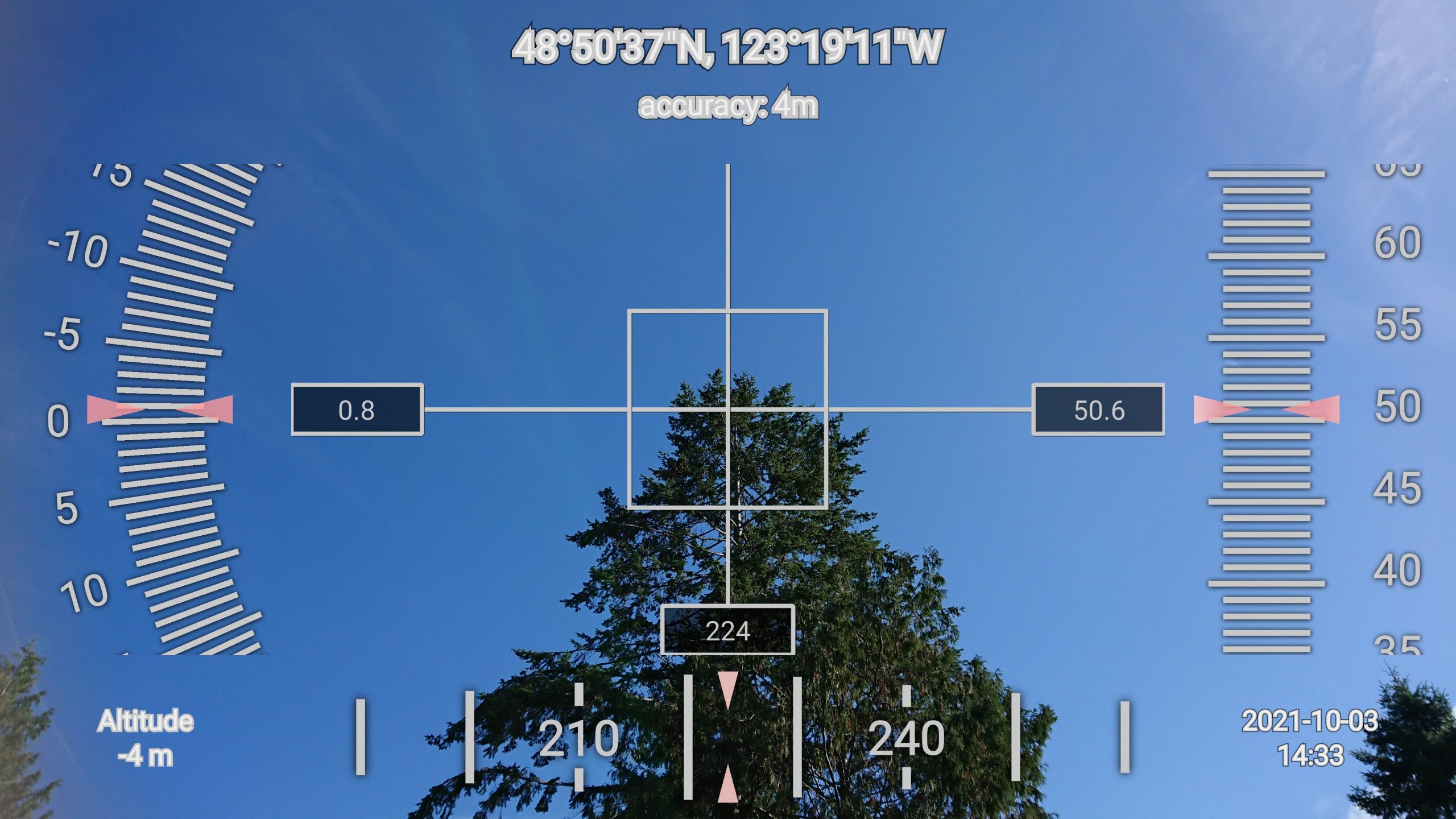
Create a Panorama Sun-Path from a 360 Photo
A similar approach can be used with panoramic images. These can be generated from a normal smartphone app by panning sideways. A 360 camera creates the best outputs as the unreliable software stitching can be omitted. Use a theodolite app to determine bearing and azimuth of features in your panorama (e.g., significant tree height) for triangulation and matching of the sun-path diagram and panorama photo.
Solar Studies using a Digital Surface Model (DSM) from Drone Lidar Data
This workflow depends on a lidar data set that has been categorized and converted to a digital elevation model (DEM). A likely file format that you will receive is a GeoTIFF file with the file extension TIF or TIFF. This is a georeferenced image file that you can open and edit in QGIS (Bewar not all TIF files are georeferenced). This DEM can represent various scenarios:
- DSM – As a digital surface model the elevations in this data represent all physical objects that did reflect the laser beam back to the lidar camera. This can be trees, cars, buildings, ground, water, etc.
- DTM – if the objects within the point cloud have been classified by the lidar operator then you are able to filter various classes of points and have the clean terrain returned to build a terrain model that you can then translate to a Revit Toposurface (see chapter “Creating a Digital Terrain Model (DTM) from GIS Data”).
The workflow described will focus on using a DSM to represent all shading objects on a site to create various solar and overshadowing studies.
Creating a 3D Mesh from a Raster DEM
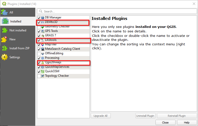
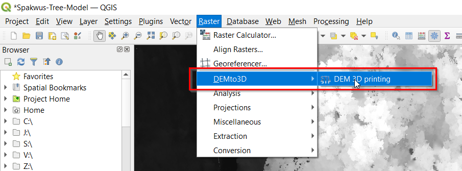
To convert the parametric raster DEM file (various shades of grey represent different elevations) to a 3D mesh model we are using a QGIS plugin called DEMto3D (https://demto3d.com/en/) and Qgis2threjs (https://qgis2threejs.readthedocs.io/en/docs/#). These tools are intended to create files for 3D printing and web publishing. Thus, some of the tools to manipulate the mesh export comes from the digital prototyping filed. The STL file describes only the surface geometry of a three-dimensional object without any representation of color, texture, or other common CAD model attributes.
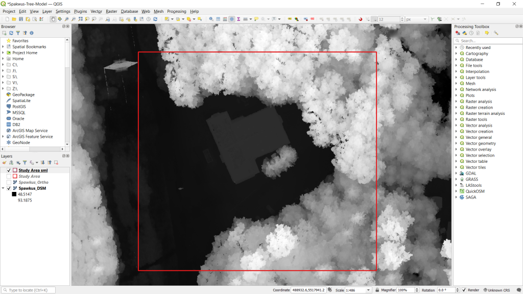
- Create a new project within QGIS and drag the DEM file (TIF or TIFF) and the aerial image file (EPW or TIF) into the map view of the program. Because both files are georeferenced, they should position exactly aligned without edits.
- Save your file into a dedicated project folder.
- Create a new layer via the menu item Layer/Create Layer/New Shapefile Layer…
- Right click this layer in the layer manager and choose Toggle Editing from the context menu.
- Draw a rectangle that represents your scope area. This rectangle will be used to clip the excess data before you export into the architectural software
- Make sure you have the necessary plugins installed
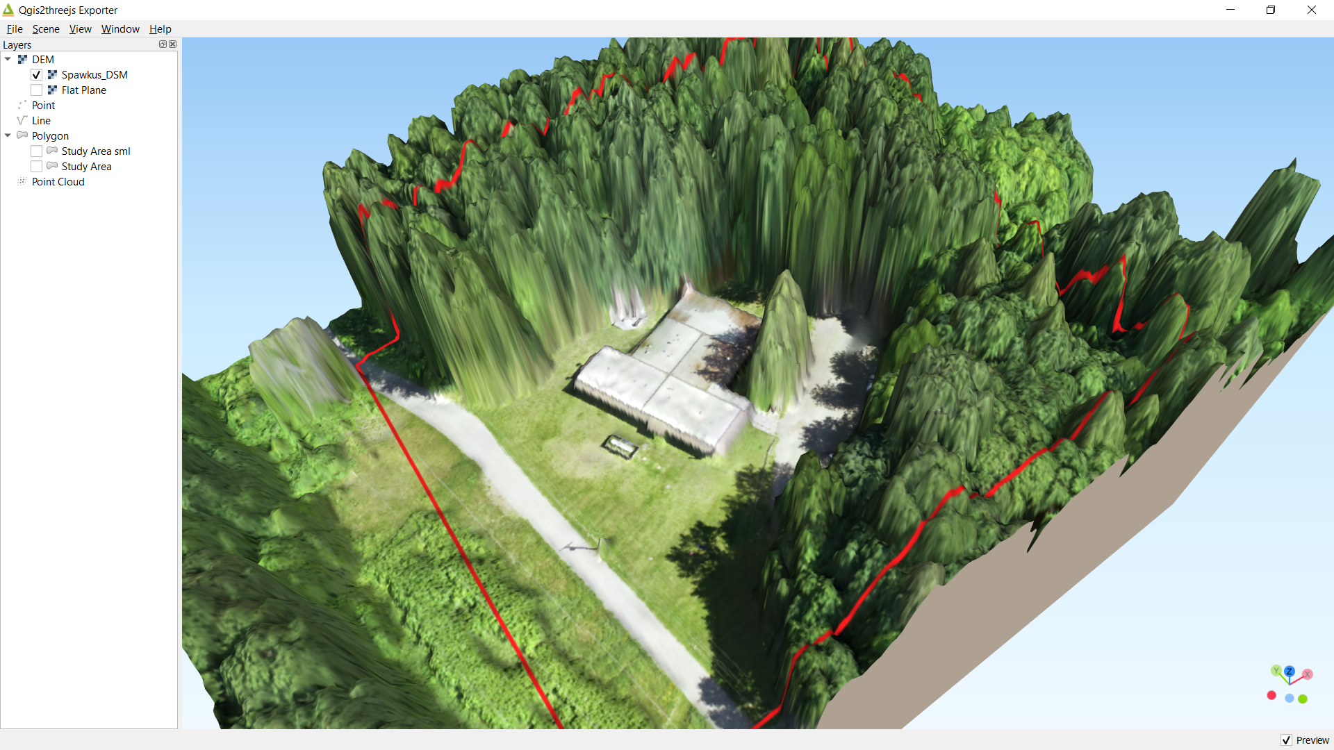
- To view the model within QGIS you can use the Qgis2threejs exporter

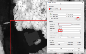
- Via the menu item Raster>DEMto3D>DEM 3D printing export prepare your mesh model export. Use your “Study Area” rectangle to set the extend or your desired mesh model. A scale of 1:1000 in our case is convenient as it allows for easily scaling it later back to 1:1 in the CAD environment just by switching from millimetre to meter. By choosing the spacing in millimetre you determine the resolution of the model (also the amount of geometry).
- Voila this is how the model looks now
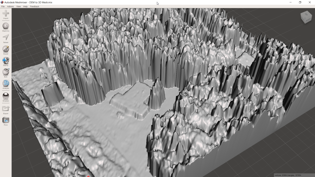
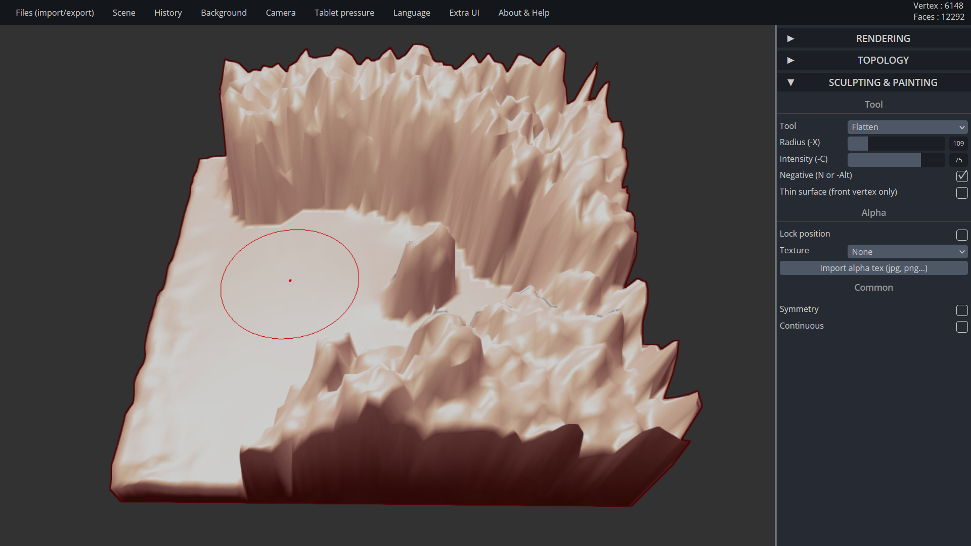
- The first digital prototyping software we use is SculptGL, this is a web based modeler that allows us to smoothen and flatten our digital surface model to erase the existing building.

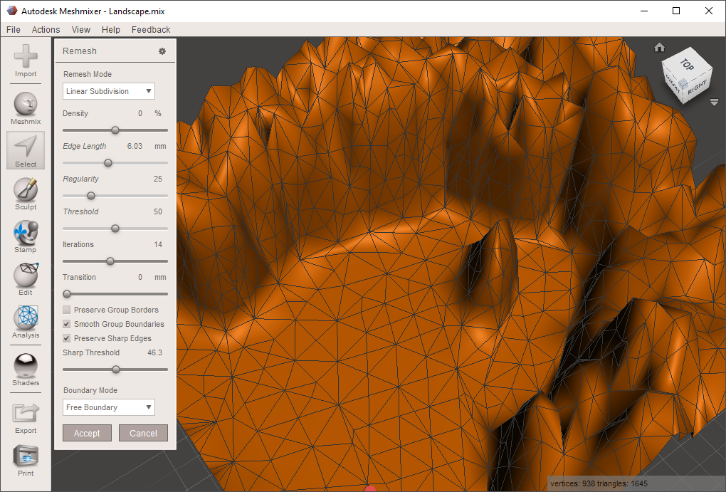
- As we want to use the geometry with solar and daylighting software, we need to find the right balance between accuracy of the surface and the amount of mesh triangles, as the complexity of the geometry will determine the time for each simulation. The program Autodesk Meshmixer proved to be the right tool to interactively reduce the mesh density
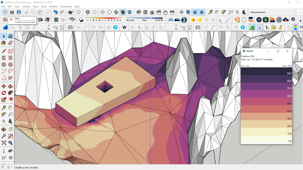
- Now the model is ready to be imported into Sketchup and design intent massing can be added
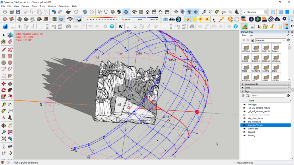
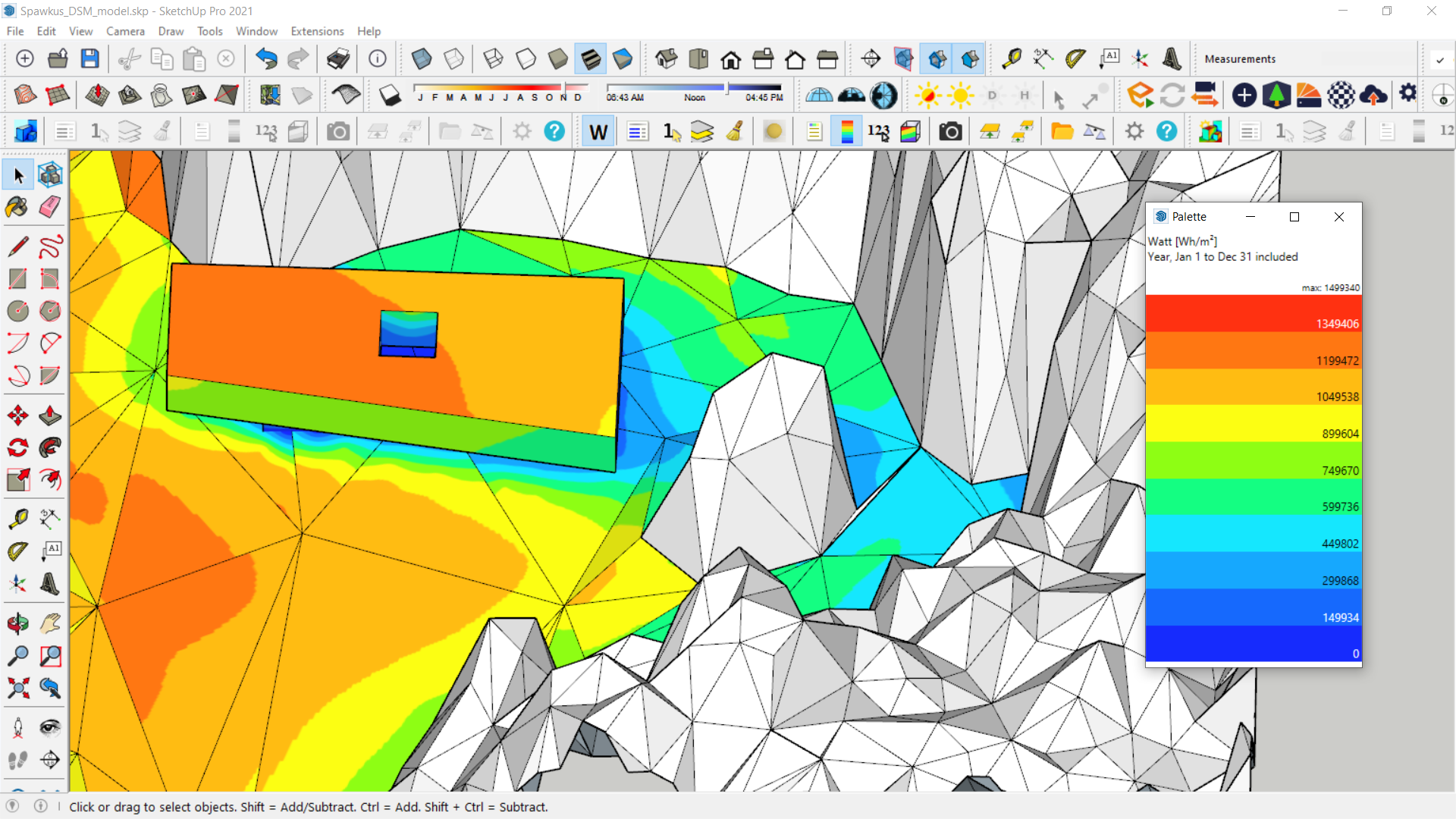
- DL-LIGHT is a SketchUp extension to study natural daylight light in architectural and urban projects. Outdoor and urban metrics like exposure to direct sun, incident energy in Watt, the sky view factor as well as indoor metrics like daylight factor and daylight autonomy are available to simulate


Dynamic Overshadowing with a Digital Surface Model
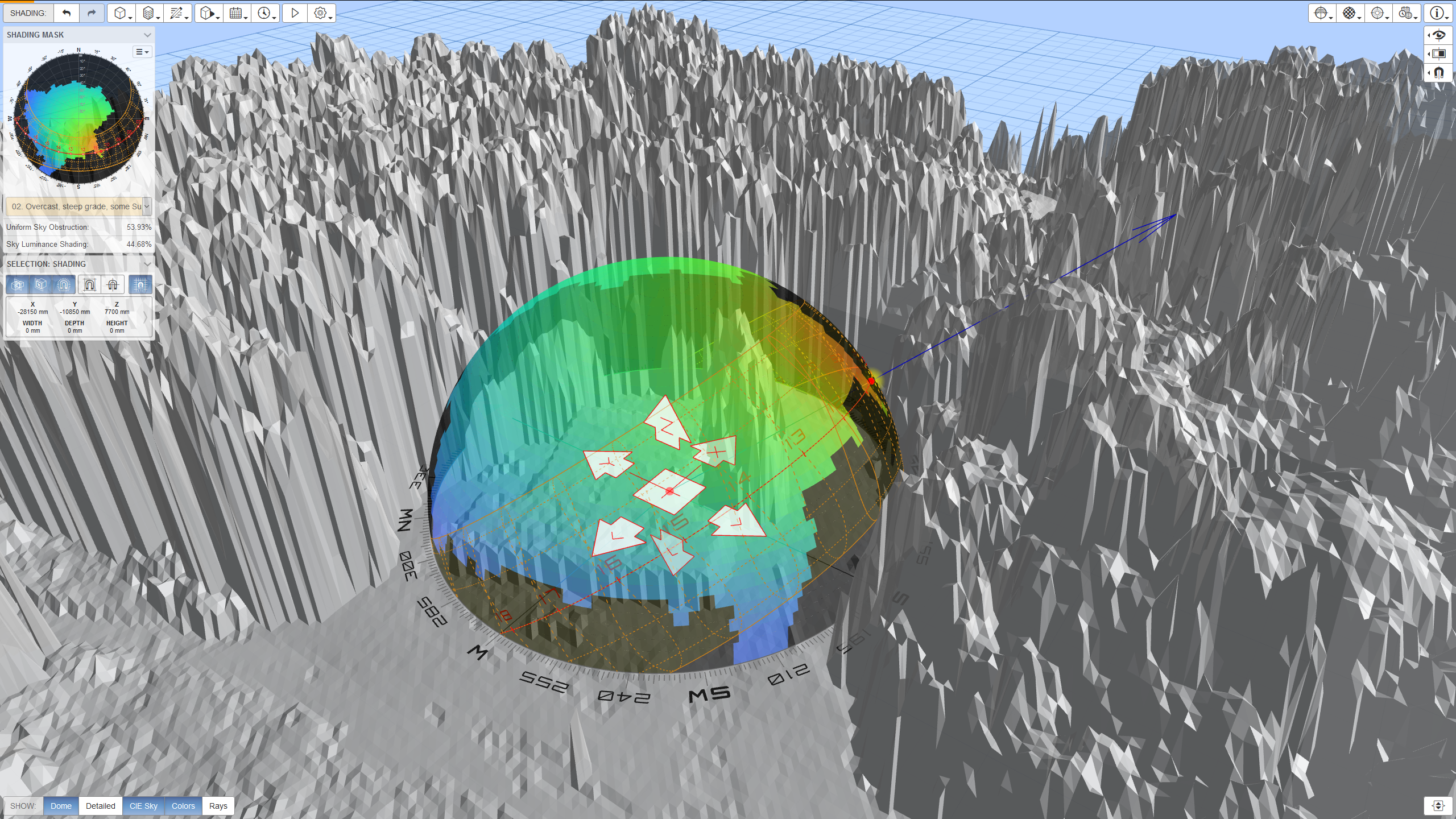
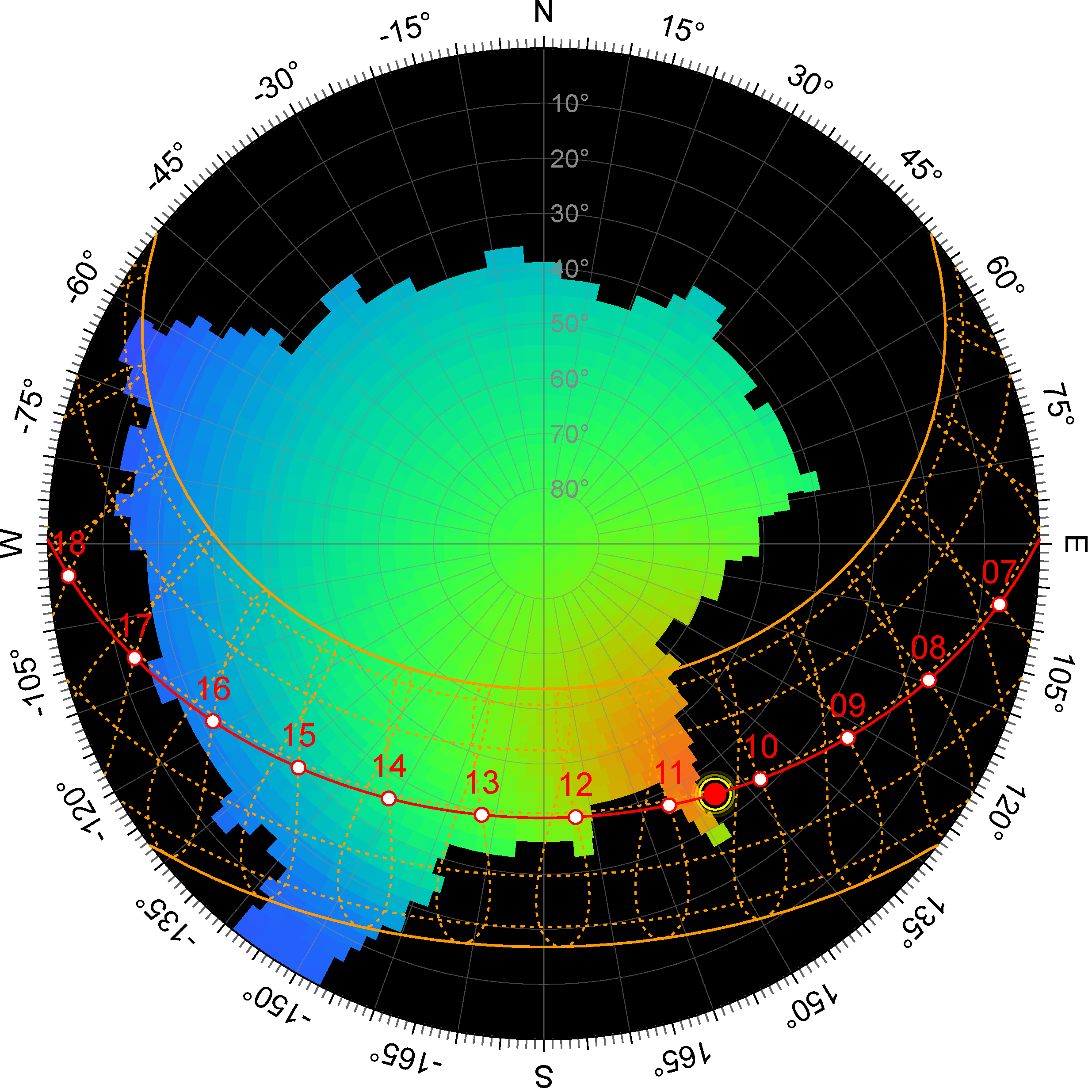
The same model can be brought into another web based Dynamic Overshadowing software by Andrew Marsh (http://andrewmarsh.com/software/shading-box-web/) to create a sky exposure mask for every point in the model. This representation is valuable to assess the availability of direct sun and overshadowing throughout the whole year in a glance.(e.g. if you are proposing an outdoor plaza, café or solar renewables).
Tools and Databases
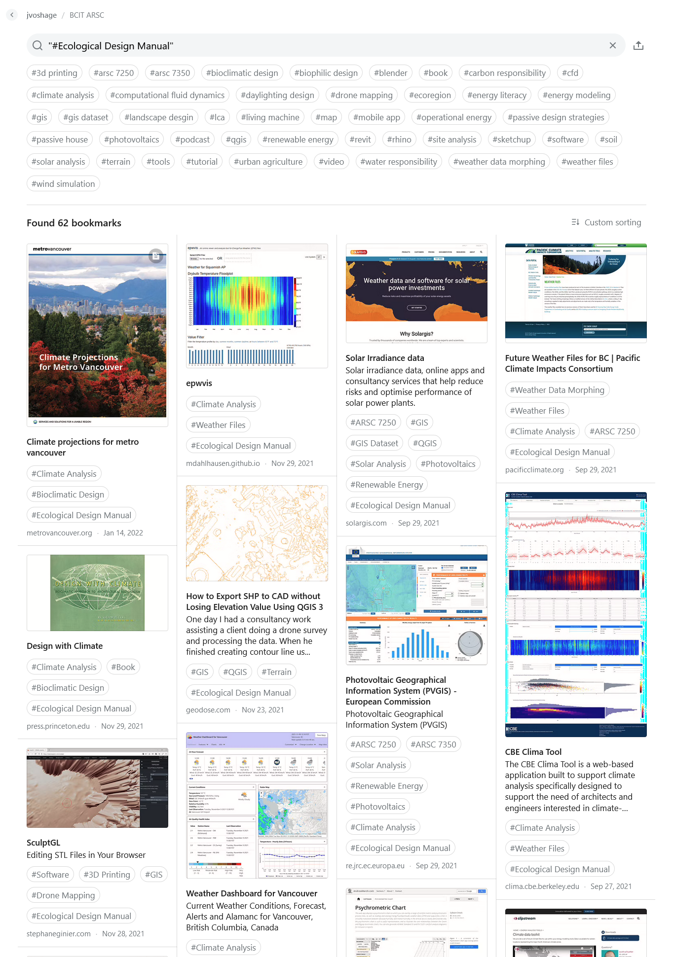
A consolidated resource listing for this chapter is available through a link list by clicking on the image below or via https://raindrop.io/jvoshage/bcit-arsc-6520383/search/sort=-sort&perpage=30&page=0&search=%22%23Ecological+Design+Manual%22
Glossary
Ecology
DEM (Digital Elevation Model)
DTM (Digital Terrain Model)
DSM (Digital Surface Model)
QGIS
GeoTIFF (file format)
LAZ/ LAZ (file format)
Revit Toposurface
SVG – Scalable Vector Graphic, XML based vector image format
STL (file format) – Standard Triangle Language, file format widely used for rapid prototyping, 3D printing
[1] https://en.wikipedia.org/wiki/Holocene
[2] The Deep Time Walk is a smartphone app / audio guided walking tour, find out more at: https://www.deeptimewalk.org/
[3] EnergyPlus™ is a whole building energy simulation program that engineers, architects, and researchers use to model both energy consumption—for heating, cooling, ventilation, lighting and plug and process loads—and water use in buildings (https://energyplus.net/).
[4] bigladder software; https://bigladdersoftware.com/epx/docs/9-3/auxiliary-programs/energyplus-weather-file-epw-data-dictionary.html#field-data-source-and-uncertainty-flags
[6] Climate Change World Weather File Generator for World-Wide Weather Data – CCWorldWeatherGen; https://energy.soton.ac.uk/climate-change-world-weather-file-generator-for-world-wide-weather-data-ccworldweathergen/
[7] Meteonorm Software; https://meteonorm.com/en/
[8] PHPP_ClimateData_SummerTemp.xlsx; https://passivehouse.com/05_service/02_tools/02_tools.htm
[9] Koppen Climate Changes from 2000-2100; How does Climate Change affect our climate types and what does that mean?; Christian DeCelle; December 8, 2020; https://storymaps.arcgis.com/stories/bffbd3c9e09f451eb7590117cdc27f1a
[10] Climate Change & Infectious Diseases Group of the University of Veterinary Medicine Vienna, Austria; http://koeppen-geiger.vu-wien.ac.at/shifts.htm
[11] The solar envelope: how to heat and cool cities without fossil fuels (https://www.lowtechmagazine.com/2012/03/solar-oriented-cities-1-the-solar-envelope.html)
Media Attributions
- Climate System
- Doughnut is licensed under a CC BY-SA (Attribution ShareAlike) license
- EPW-in-Notepad++
- EPW in MS Excel
- EnSimS-EPW Map-Squamish_01
- EnSimS-EPW Map-Squamish_02
- EnSimS-EPW Map-Squamish_03
- Davis_Instruments_weather_station_-_detail is licensed under a CC BY-SA (Attribution ShareAlike) license
- CAN_BC_Squamish.AP.712070_CWEC2016_HadCM3-A2-2080 in Elements
- Climate-Analysis-Poster © Jens Voshage is licensed under a All Rights Reserved license
- Andrew-Marsh_2D-Data Viewer_01
- Andrew-Marsh_2D-Data Viewer_02
- Andrew-Marsh_Weather-Data Viewer_01
- Climate -Consultant_Windrose_Spring-Summer-Fall
- Andrew-Marsh_Psychrometric-Chart
- Climate-Consultant_Psychrometric-Chart
- Wikipedia_Squamish-Precipitation
- Rainwater-Harvesting-Calc
- PCIC Future Precipitation
- Andrew-Marsh_2D-Data Viewer_03
- Climaplus – Temperatures_TMY-2080
- Andrew-Marsh_Weather-Data Viewer_02
- Andrew-Marsh_Weather-Data Viewer_03
- CCWorldWeatherGen_Squamish
- PHI-Summer-Tool
- Climate-Atlas-of-Canada_04
- Climate-Atlas-of-Canada_01
- Climate-Atlas-of-Canada_05
- Sketchup-oob-terrain
- Blender-OSM_Granville-Island
- QGIS-UI
- QGIS-Contours-01
- QGIS-Contours-02
- QGIS-Contours-03
- QGIS-Tutorial_01
- QGIS-Tutorial_02
- QGIS-Tutorial_03
- Revit-Toposurface
- Revit-Toposurface-with-Point-Cloud-Overlay
- Enscape-01
- Enscape-02
- Enscape-03
- udeuschle.de – Creating a 360 DEM Panorama Image
- Panoramic DEM with Sun-Path Diagram Superimposed
- Geocam01
- Cheakamus-Panorama-Sunpath-Cartesian_Photo
- QGIS-Revit_DEM&Study-Area
- QGIS Plugins
- QGIS-Revit_DEM&Study-Area-Qgis2threejs
- QGIS-Revit_DEM 3D printing plugin
- DEM to 3D – Export
- Meshmixer – DEM to 3D Mesh.mix
- SculptGL
- Autodesk Meshmixer.mix
- Sketchup-01
- DL-Light-in-Sketchup_01
- DL-Light-in-Sketchup_02
- Andrew-Marsh_Dynamic-Overshadowing_01
- Andrew-Marsh_Dynamic-Overshadowing_02
- Tools-Databases
- https://climateatlas.ca/climate-atlas-version-2 ↵