Spatial Model Skill Assessment
Spatial Fitting
When fitting a model to data, two main processes are involved: the modification of parameters to better-fit observational data (called model calibration), and the comparison of predicted results with independent observations to validate results (or model validation). These processes are frequently done together to evaluate the performance of a model. With increasing spatial data available, the separation between calibration and validation should ideally become standard practice in Ecospace modeling.
Advancing Towards Calibration of Ecospace
Contrary to the temporal model Ecosim, Ecospace model calibration is still rarely systematically executed due to the complexity of parameters involved, the need for large space-time datasets, and lack of computing power [1][/footnote]. The majority of Ecospace users are manually tuning key parameters to obtain reliable distribution of species on the basis of visual inspection and confrontation with available spatial data. Some advances have been made by running Ecospace outside the user interface, using R or Python, to systematically evaluate parameter sensitivities and search for values that improve model fit [2]Vilas, D., 2022. Spatiotemporal Ecosystem Dynamics on the West Florida Shelf : Prediction, Validation, and Application to Red Tides and Stock Assessment. University of Florida. https://doi.org/10.1038/s41598-023-29327-z[/footnote]. In addition to tuning Ecospace parameters (as described in previous sections), also several Ecosim parameters could be changed during the tuning process. For example, vulnerability multipliers are calculated based on biomasses averaged over the entire spatial domain. When a fitted Ecosim model is migrated into Ecospace the calibrated vulnerability multipliers of some species might be too high for species that are confined to limited domains (restricted depth range, specific substrates, etc.) in Ecospace due to its spatial overlap with that of its predators and of the main target fishery. In cases such as these, Ecosim vulnerability multipliers (by predators or by predator-prey interactions) need to be manually tuned to reach the temporal-spatial stability of these species.
When dispersion rates are low, they might help to concentrate a species into stable hot spots or conversely, when high, dispersal rates might allow excessive dispersal of biomass in the domain. Consequently, higher dispersal rates tend to lead to models that better fit observational data but that can become ecologically unrealistic. The dispersion rate also influences the resulting effects of MPAs, since high dispersal might predict large spill-over from areas of protection and hamper biomass rebuilding thus reducing the benefits for highly exploited species. Iterative testing the effects of the parameter values such as dispersal rates and vulnerabilities on spatial distribution of species (based on simple visual inspection) under e.g. MPAs setting can be done manually as part of the calibration process [3].
Another component of spatial calibration is adjusting the response curves to environmental drivers (e.g., temperature, depth, dissolved oxygen) to better represent the aggregation of species, i.e., to resemble the aggregation in favorable areas in terms of environmental conditions [4]. Species distributions obtained from species distribution models or SDMs [5] can be used to either force the habitat capacity of a species [6] or can be used to compare with Ecospace model outputs for validation purposes: this is often done off-line, which allows for testing of the efficacy of tuning done manually, while not using optimization routines to create a better fit [7].
To tune the cost of fishing and the distribution of fishing effort in Ecospace, distance from ports can be compared with, for example, analysis of Vessel Monitoring Systems (VMS) or Automatic Information System (AIS; [8]). Furthermore, administrative boundaries (EEZ boundaries), gear specific costs and habitat preferred for fishing (e.g., trawling avoiding rocky areas) are additional parameters that can improve accuracy of fisheries distribution over space. However, some specific spatial behavior of fishermen not directly related to the abundance and value of target species (e.g., fishery ground fidelity) might be quite difficult to represent. Overall, lacking better features to reproduce fishers’ behavior, Ecospace assumes that all fleet elements have complete knowledge of distribution of the target species. Connecting Ecospace to an explicit fisheries behavior model is a development of interest for the future.
Spatial Validation
Validation is the process of assessing whether a parameterized and calibrated model effectively performs as it should. In other modelling context, traditionally the data pool is split in a set only used for calibration, and another set only used to finally validate the model with a proportion that can range from 50-50 to 80-20. Alternatively, completely different sets of data can be used for the validation. The validation serves as a proof of model skills. Such formal exercise is not often performed in Ecospace, while in the context of progressive application of EwE and Ecospace in operational context it is ideal to deliver a systematic validation of the models, and some examples of how this has been done are provided below.
Hotspot Analysis
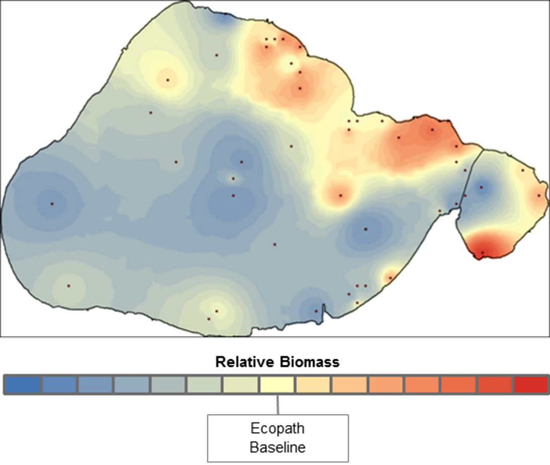
The use of existing telemetry data on particular species of interest is one data source that has been under-utilized in developing validation methods for spatial-temporal models. Ecospace includes a plug-in called the XY Hotspot Tool, which allows the user to include the frequency of detection of species from telemetry data and calculates the error between predicted and observed between telemetry data and Ecospace output maps. One unpublished example of this approach, called the XY Hotspot Analysis, was tested on Spotted Seatrout (Cynoscion nebulosus) in Lake Pontchartrain, Louisiana, USA. From 2012 to 2014, the movements of 211 Spotted Seatrout were monitored using an acoustic array composed of 90 autonomous receivers. The “pings” recorded on the receivers were converted to biomass using a novel methodology and then using various GIS interpolation techniques, species distribution maps were created at monthly time steps. Then, using the XY Hotspot tool, the prediction error between the maps output by the Ecospace model and the maps developed using the telemetry data were calculated (Figure 1).
Using Regional Observations to Validate Distribution Patterns
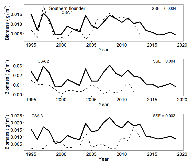
Validation often requires two datasets covering the same area (one for model creation, one for model validation), which is rare to have, e.g., two monitoring programs covering the same area. However, when a dataset has not been initially used to determine the spatial distribution of species, it can be used to validate distribution patterns. This is often the case with EwE models. Survey data that cover the whole model area can be used to create a representative snapshot of the ecosystem (the Ecopath model). By creating regions within the Ecospace model area, averaged output of subsections can be generated. Time series of this output can be compared with survey data time series from field sites within that same subsection (see De Mutsert et al. [9] [10] for examples). Goodness-of-fit metrics can be applied outside of the model interface. This is an easy non-spatial solution to validate how the habitat capacity framework distributes species based on habitat affinity and environmental preferences when spatial features are included in the model with response curves (Figure 2).
Multi-Model Comparisons
Statistical analysis of species occurrences and their relationships with associated environmental factors is used to predict how likely a species is to occur in unsampled locations as well as future conditions. However, environmental factors alone may not be sufficient to account for species distribution. Other ecological processes including species interactions (such as competition and predation) and the impact of human activities, may affect the spatial distribution of a species. Novel techniques have been developed to take a more holistic approach to estimating species distributions, such as Bayesian Hierarchical Species Distribution model (B-HSD model) and mechanistic food-web models using the HFC model. Coll et al. (2019) used both species distribution and spatial food-web models to predict the distribution of European hake (Merluccius merluccius), anglerfishes (Lophius piscatorius and L. budegassa) and red mullets (Mullus barbatus and M. surmuletus) in an exploited marine ecosystem of the Northwestern Mediterranean Sea. They explored the complementarity of both approaches, comparing results of food web models previously informed with species distribution model results, aside from their applicability as independent techniques. The study showed that both B-HSD and E-HFC model results were positively and significantly correlated with observational data. Predicted spatial patterns of biomasses showed positive and significant correlations between modeling approaches and were more similar when using both methodologies in a complementary way: when using the E-HFC model previously informed with the environmental envelopes obtained from the B-HSD model outputs, or directly using niche calculations from B-HSD models to drive the niche priors of the Ecospace HFC [11].
Adaption
The chapter is adapted, with permission, from:
De Mutsert K, Marta Coll, Jeroen Steenbeek, Cameron Ainsworth, Joe Buszowski, David Chagaris, Villy Christensen, Sheila J.J. Heymans, Kristy A. Lewis, Simone Libralato, Greig Oldford, Chiara Piroddi, Giovanni Romagnoni, Natalia Serpetti, Michael Spence, Carl Walters. 2023. Advances in spatial-temporal coastal and marine ecosystem modeling using Ecopath with Ecosim and Ecospace. Treatise on Estuarine and Coastal Science, 2nd Edition. Elsevier.
- Romagnoni, G., Mackinson, S., Hong, J., Eikeset, A.M., 2015. The Ecospace model applied to the North Sea: Evaluating spatial predictions with fish biomass and fishing effort data. Ecological Modelling 300, 50–60. https://doi.org/10.1016/j.ecolmodel.2014.12.016 [footnote]Steenbeek, J., Buszowski, J., Chagaris, D., Christensen, V., Coll, M., Fulton, E.A., Katsanevakis, S., Lewis, K.A., Mazaris, A.D., Macias, D., de Mutsert, K., Oldford, G., Pennino, M.G., Piroddi, C., Romagnoni, G., Serpetti, N., Shin, Y.-J., Spence, M.A., Stelzenmüller, V., 2021. Making spatial-temporal marine ecosystem modelling better – A perspective. Environmental Modelling & Software 145, 105209. https://doi.org/10.1016/j.envsoft.2021.105209 ↵
- [footnote]Vilas, D., Buszowski, J., Sagarese, S., Steenbeek, J., Siders, Z., Chagaris, D., 2023. Evaluating red tide effects on the West Florida Shelf using a spatiotemporal ecosystem modeling framework. Scientific Reports 13, 2541. ↵
- (e.g., Romagnoni et al. 2015, op. cit.) ↵
- Vilas, D., Chagaris, D., Buszowski, J., 2020. Red tide mortality on gag grouper from 2002-2018 generated by an Ecospace model of the West Florida Shelf. SEDAR, North Charleston SC. ↵
- Panzeri, D., Bitetto, I., Carlucci, R., Cipriano, G., Cossarini, G., D’Andrea, L., Masnadi, F., Querin, S., Reale, M., Russo, T., Scarcella, G., Spedicato, M.T., Teruzzi, A., Vrgoč, N., Zupa, W., Libralato, S., 2021. Developing spatial distribution models for demersal species by the integration of trawl surveys data and relevant ocean variables., in: Copernicus Marine Service Ocean State Report, Issue 5. pp. s114–s123. ↵
- Püts, M., Taylor, M., Núñez-Riboni, I., Steenbeek, J., Stäbler, M., Möllmann, C., Kempf, A., 2020. Insights on integrating habitat preferences in process-oriented ecological models – a case study of the southern North Sea. Ecological Modelling 431, 109189. https://doi.org/10.1016/j.ecolmodel.2020.109189 ↵
- Coll, M., Pennino, M.G., Steenbeek, J., Sole, J., Bellido, J.M., 2019. Predicting marine species distributions: Complementarity of food-web and Bayesian hierarchical modelling approaches. Ecological Modelling 405, 86–101. https://doi.org/10.1016/j.ecolmodel.2019.05.005 ↵
- Russo, T., D’Andrea, L., Parisi, A., Cataudella, S., 2014. VMSbase: An R-Package for VMS and Logbook Data Management and Analysis in Fisheries Ecology. PLOS ONE 9, e100195. https://doi.org/10.1371/journal.pone.0100195 ↵
- De Mutsert, K., Lewis, K.A., Buszowski, J., Steenbeek, J., Milroy, S., 2017. 2017 Coastal Master Plan Modeling: C3-20-Ecopath with Ecosim. Coastal Protection and Restoration Authority. ↵
- De Mutsert, K., Lewis, K., Milroy, S., Buszowski, J., Steenbeek, J., 2017. Using ecosystem modeling to evaluate trade-offs in coastal management: Effects of large-scale river diversions on fish and fisheries. Ecological Modelling 360, 14–26. https://doi.org/10.1016/j.ecolmodel.2017.06.029 ↵
- Coll et al., 2019, op. cit ↵
