Spatial Distribution
In Ecospace, a modeled area is represented by a grid of equally sized cells, where each cell has the basic Ecosim trophic linkage dynamics and other components of ecosystem dynamics, and cells are linked through biomass flows associated with spatial mixing processes. Cells with ecosystem dynamics need a number of descriptors to define how specific ecosystem components and fishing fleets can utilize the cell.
In the original 2008 version of the Ecospace model, each cell with ecosystem dynamics would be assigned to a single, discrete habitat type, and functional groups would be assigned to preferred habitats (Christensen and Walters, 2004; Pauly et al., 2000; Walters et al., 1999). Fishing fleets would be allowed to fish over specific habitats, or could be blocked from fishing in no-take zones (Walters, 2000). Moreover, relative variations of the primary productivity and of costs of fishing across space (but fixed in time) could be incorporated to influence the spatial distribution of the food web and fishing effort, while the model accounts for species movement and other behavioral aspects.
In the 2008 version, habitat structures with associated impact on biomass distributions and trophic interactions were represented by a binary habitat use pattern, with each spatial cell being either entirely suitable – or entirely unsuitable – for species/functional groups. Therefore, the original version of Ecospace assumed homogeneous conditions within each spatial cell, and local but possibly relevant variations within cells could not be represented (Christensen et al., 2014). In addition, a major shortcoming in this original Ecospace configuration was the limited support to include environmental variability as the model ran (Steenbeek et al., 2013).
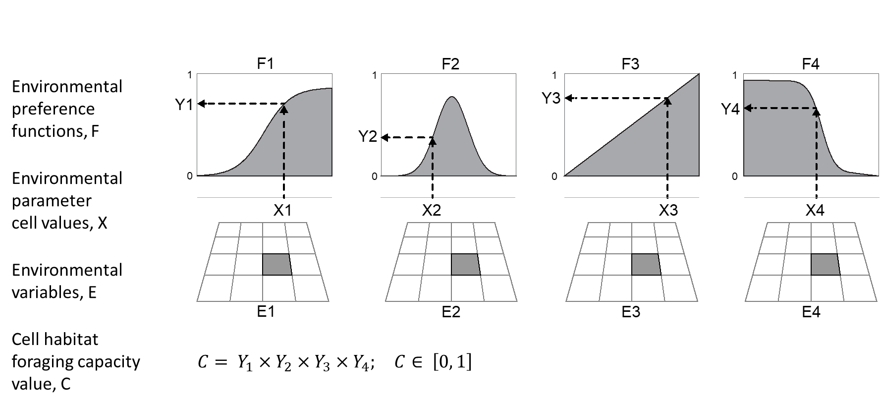
Functional groups in Ecospace disperse throughout the map based on cell suitability, representing the tradeoff between being able to eat and the risk of being eaten, where differences in cell suitability define the likelihood of a species moving to a neighbouring cell (Christensen et al., 2014). In 2013, Ecospace version 6.3 introduced the Habitat Foraging Capacity (HFC) model that computes the foraging arena size in a cell (Christensen et al., 2014). The HFC contains two main methods, described below, that can be used to define the foraging arena size, or foraging capacity which can be used individually or in combination (Fig. 4).
The Habitat Foraging Capacity (HFC) model consider the cumulative effects of physical, oceanographic, and environmental conditions (such as depth, bottom type, temperature, salinity, oxygen concentrations and primary production) onto species distributions (Christensen et al., 2014). The HFC model defines a continuous relative habitat capacity for each functional group in each cell (Christensen et al., 2014), and the proportion of a cell that functional groups can use became a continuous value from 0 to 1, allowing for the inclusion of as many environmental factors as needed to define the foraging capacity of a cell for a species (Fig. 1).
Habitat Affinity
The first method is the legacy Ecospace habitat affinity modus, where the user defines habitat that typically relate to types of substrate relevant to the ecosystem, and how functional groups prefer each different type of habitat. Typically, 5-10 habitat types are used, although there can be many more. For each type of habitat (e.g., sand, rock, seagrass, mud, gravel, etc.) there is an accompanying habitat map that expresses the fraction of cell coverage by that habitat type on a scale of 0 to 1, where 0 indicates no presence and 1 indicates a cell covered entirely by that habitat.
Per functional group, users can quantify how preferred the habitat is for each given functional group that relies on habitats. Preference values range from 0 to 1, where 0 indicates no preference, and 1 optimal preference. Per cell, Ecospace can thus have patches of multiple habitats. The combined presence of habitats and individual habitat preferences leads to a total habitat suitability factor between 0 and 1 for any given functional group, across the map (Püts et al., 2020; Walters et al., 1999). Note that habitats can also be used to indicate vertical structures (e.g., Steenbeek et al., 2020). The sum of habitat areas used by group in a cell should sum to, and not exceed 1.
Environmental Preferences
With the introduction of the Habitat Foraging Capacity model (Christensen et al., 2014), Ecospace gained a second option to calculate cell foraging suitability through the presence of environmental drivers and functional responses to these drivers. The “environmental preferences” model is similar to a habitat suitability index model that is widely used in spatial ecology (Rushton et al., 2004). Users can define any number of environmental drivers that are known to affect the distribution of parts of the modeled food web. For each defined environmental driver (sea surface temperature, wave action, low frequency noise, bottom dissolved oxygen, salinity etc.) Ecospace incorporates a spatial map that describes how the driver is distributed across the modeled area. A functional response curve, unique to each group and shared with Ecosim (see section 1.4.2), which defines the environmental effect of the driver to each impacted group also needs to be entered. One advantage of the “environmental preferences” model is that the same environmental driver data can be used across a number of functional groups, with response curves being used to specify group tolerances to, or preferences for, specific environmental conditions. The spatial-temporal framework added the ability to change the maps with environmental conditions over time (Steenbeek et al., 2013).
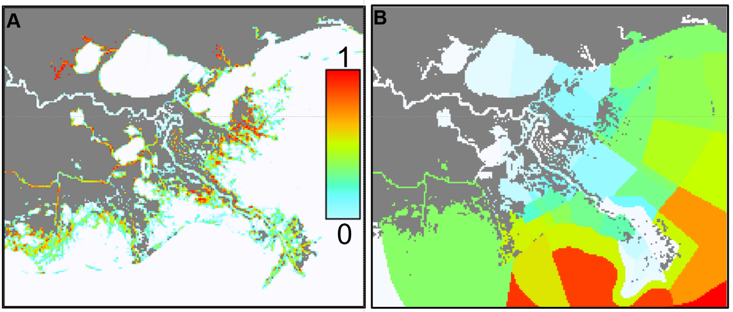
The HFC model considers “habitat affinity” and “environmental preferences” and solves most of the problems of the old habitat affinity (only) model. With the release of EwE 6.5, the combined use of habitats and environmental sensitivities is a per-group setting. This means that users have the freedom to control whether the utilization of space by a given group is driven by habitat affinity, by environmental preferences, or both (see Fig. 5 for example).
Recommendations
As the user develops the habitat and environmental driver maps and response curves necessary to define how groups use the modeled space, it is advisable to start with the few environmental features that are most important for defining the distribution. Complexity can be built gradually, with less important environmental features being added subsequently until a realistic biomass distribution of groups is achieved. This is to avoid the problem of driver temporal and spatial correlation: their simultaneous application can result in an overemphasized effect on species distribution (Amodio, 2015; Serpetti et al., 2016). For example, temperature and depth may each play a role in establishing the spatial domain inhabited by a species or group, but these two environmental features are in many cases not independent. It is not trivial to disentangle these environmental effects, and some authors suggest the prior use of multivariate or spatial statistical approaches to determine appropriate coefficient weightings (Coll et al., 2019; Grüss et al., 2018) or selection and exclusion in case of strong correlation, a common practice for example in GAM modeling (Panzeri et al., 2021; Serpetti et al., 2016).
Adaption
The chapter is in part adapted, with permission, from:
De Mutsert K, Marta Coll, Jeroen Steenbeek, Cameron Ainsworth, Joe Buszowski, David Chagaris, Villy Christensen, Sheila J.J. Heymans, Kristy A. Lewis, Simone Libralato, Greig Oldford, Chiara Piroddi, Giovanni Romagnoni, Natalia Serpetti, Michael Spence, Carl Walters. 2023. Advances in spatial-temporal coastal and marine ecosystem modeling using Ecopath with Ecosim and Ecospace. Treatise on Estuarine and Coastal Science, 2nd Edition. Elsevier.
