Introduction

The Ecoengineer plugin is designed for predicting the spatial spread of functional groups in benthic ecosystems with at least one autogenic ecosystem engineer: an animal or plant that uses its own body to change an environment and affect the access of other species to resources ^[1]. Ideally, the engineering species should be hard in structure. In the accompanying publication Sadchatheeswaran et al. ^[2], mussel and barnacle beds, which dominated the intertidal area considered, were used.

The Ecoengineer plugin for Ecospace, the spatial‐temporal modelling routine of Ecopath with Ecosim or EwE (Christensen and Walters 2004), is publicly available with EwE version 6.6.5 and onward.

Using Ecoengineer

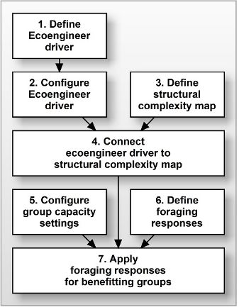
Setting up Ecoengineer dynamics in a EwE model thus requires the following:

• A balanced Ecopath model, with an Ecosim and Ecospace scenario
• One or more eco‐engineer functional groups present in the ecosystem model
• Definition of the empirical relationship between ecoengineer biomass and structural complexity
• Definition of an Ecospace environmental driver map that will receive the amount of structural complexity
• Definition of functional responses for all functional groups that are affected by this new environmental driver

Figure 1 outlines how to achieve this in the EwE desktop software. The steps are described in detail, below.

Preparation: Set Up a Temporal‐Spatial Model

In EwE, create a balanced Ecopath model of the ecosystem that represents the first year of biomass time series of ecosystem engineers. Make sure ecosystem engineers are explicitly represented by at least one functional group. Run the model for a set number of years in Ecosim, with a time series to drive the biomass of functional groups over time. In Sadchatheeswaran et al.^[3] , the time series was run for 35 years (1980 to 2015), and the initial biomasses of the alien ecosystem engineer groups started low and were forced at each annual time step, rather than use fitted data, as per the recommendations of Langseth et al.^[4]. The biomasses of the native functional groups in the time series can be used to fit the model to observed data. The model is then ready for Ecospace, the spatial‐temporal modelling routine.

In Ecospace, open and name a new scenario that should automatically run for the total number of years dictated in Ecosim. In Maps (Ecospace>Input), create a base map that matches the size of the study area ^{[5] [6]}. If possible, also create depth (or zonation) and habitat layers on this map to drive functional group biomass to preferred areas on the map, based on observational data.

Step 1: Enable Ecoengineer Dynamics

The first step to enabling ecosystem engineer dynamics is to define the empirical relationship between engineering species biomass and derived structural complexity. We implemented this connection through the Ecospace ‘external data connections’ system (Steenbeek 2021), where the Ecoengineer plug‐in acts as an intermediate calculator that calculates structural complexity while Ecospace executes ^[7].

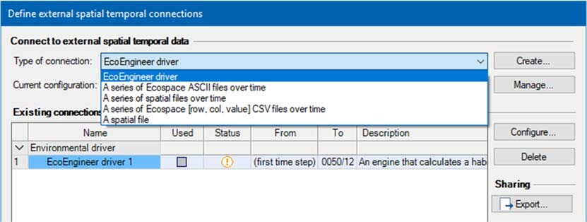
From the menu bar, go to Ecospace > Define External Data Connections. Under Connect to external spatial temporal data select the EcoEngineer driver and press Create. This new connection should now be present under the Existing connections.

The next step is to parameterize the relationship between the ecosystem engineer biomasses and the structural complexity (Figure 3).

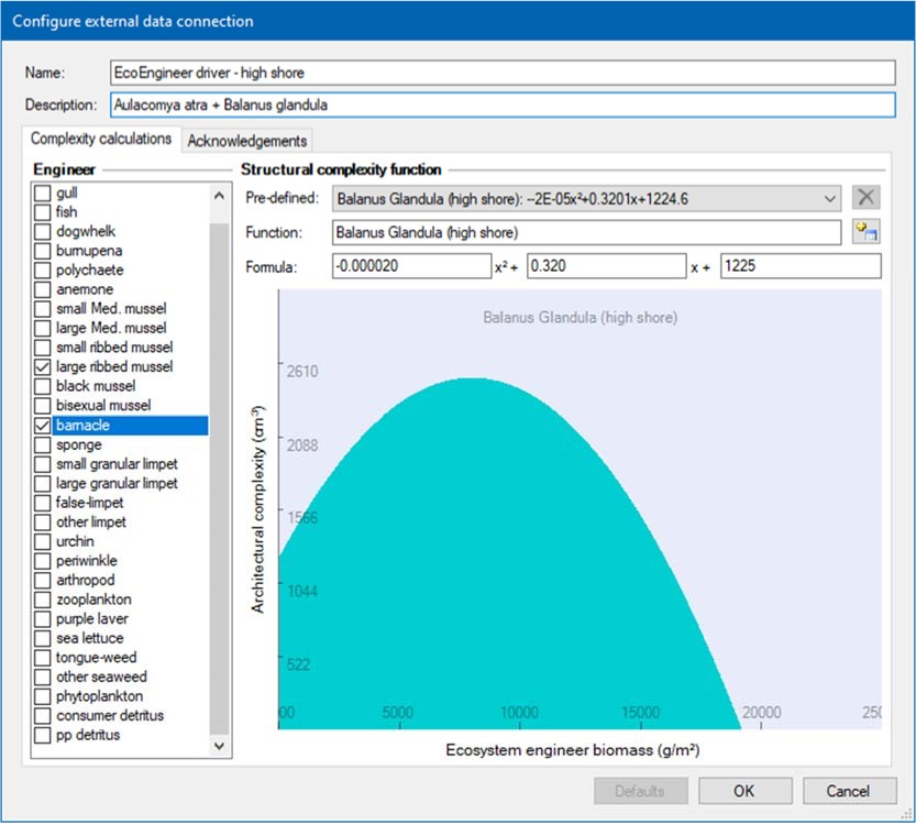
Make sure the new connection is selected and press Configure.

First, provide your Ecoengineer set‐up with an intuitive name and an optional description.

In the Complexity calculations tab, choose an ecosystem engineer in the left frame. In the right frame, select a predefined function of how structural complexity changes as a function of ecosystem engineer biomass (if suitable). Otherwise define formulae based on observational data, by entering parameters for a, b and c of y = ax2+bx+c, where y is structural complexity (cm3) and x is engineering biomass (g m‐2). Derivation of these calculations is discussed in Sadchatheeswaran et al. ^[8]. Repeat for all ecosystem engineers.

Step 3: Define Ecoengineer as an Environmental Driver Map

Once empirical relationships between habitat building biomasses and structural complexity are defined, Ecospace needs to be informed of how individual functional groups respond to structural complexity. First, a new environmental driver map is needed to receive the spatial‐ and temporally varying structural complexity to drive structural complexity‐related functional responses.

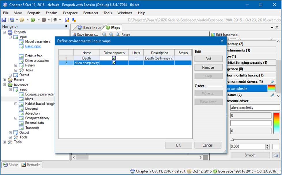
 In the Menu bar, select Ecospace > Define Environmental Driver maps. Add and name a new environmental driver. For illustration, in Figure 4, the driver was named ‘alien complexity’. The driver will show up under Environmental drivers in the Map window of Ecospace.

The environmental driver map, defined in Step 3, must receive the ecosystem engineer calculated complexity, defined in Steps 1 and 2. This is achieved by connecting the external driver (defined in step 2) to the environmental driver (defined in step 3). This will make the alien complexity map vary in response to changing habitat‐building biomasses.

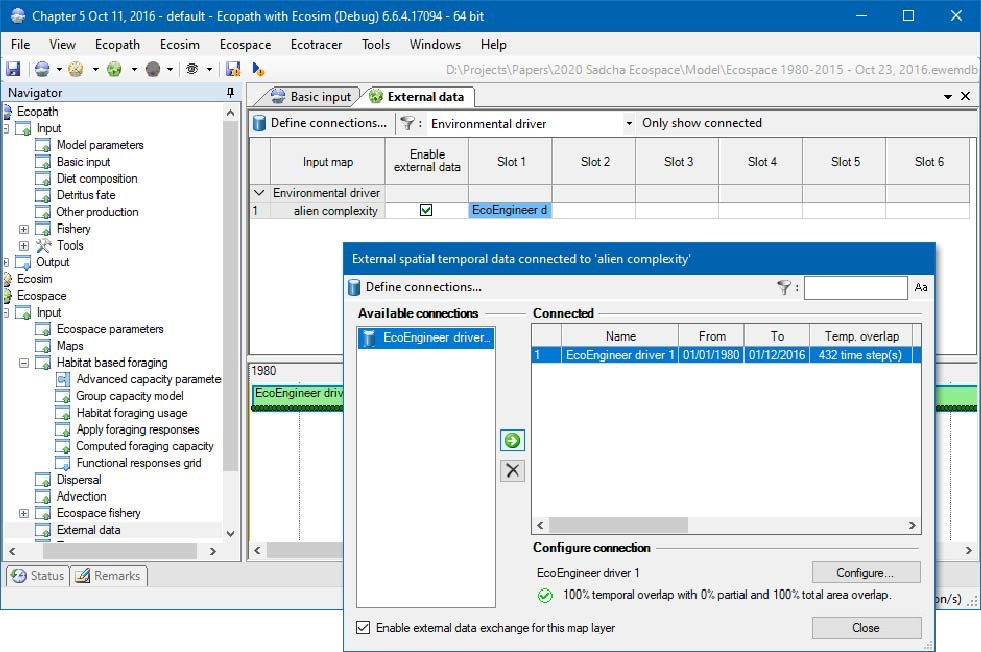
In the Navigator window, select Ecospace > Input > External data. In the main window, there will be several input maps; select Environmental drivers. Click on the column marked Slot 1 in the row marked alien complexity (for illustration) (Figure 5).

In the window that pops up, under available connections, select the Ecoengineer driver that you created and configured in steps 1 and 2, and click the right arrow button to connect the driver to the alien complexity map. Close the window.

The Ecoengineer driver is applied properly when a green time series line is present in the external data window.

Make sure that Ecospace niche model, the habitat foraging capacity model, knows which functional groups must respond to environmental drivers.

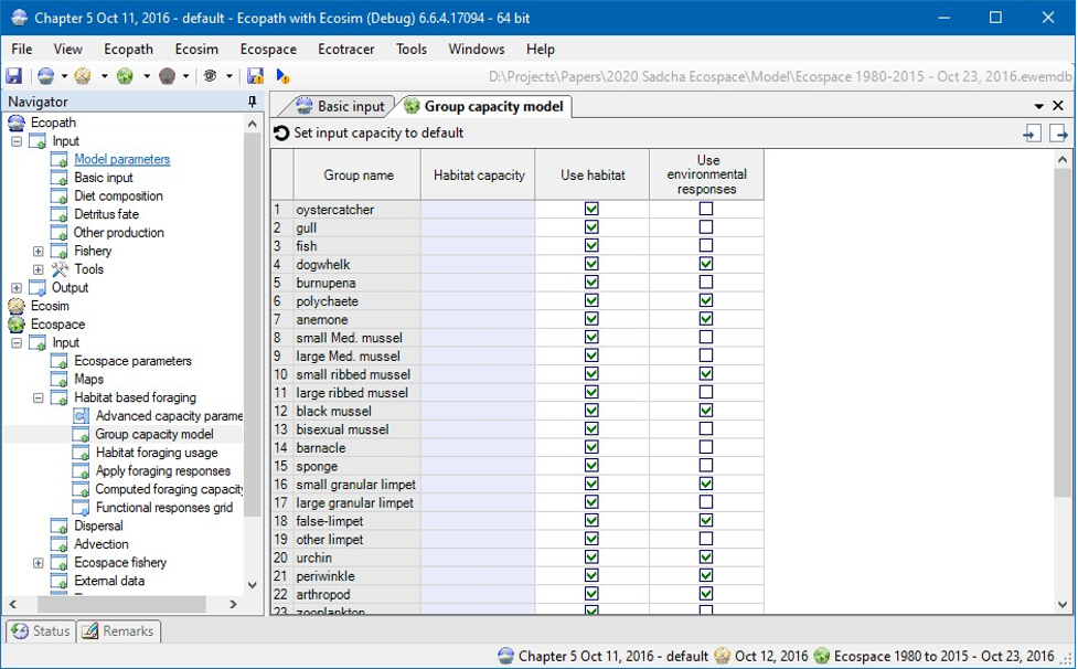
 In the Navigation window, choose Ecospace > Input > Habitat based foraging > Group capacity model. Ensure that the option “use environmental responses” is checked for all functional groups that are affected by structural complexity (Figure 6).

Next, define how individual functional groups are affected by structural complexity.

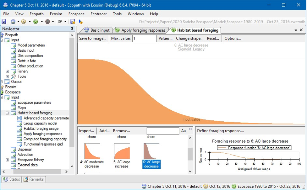
In Ecospace > Input > Habitat based foraging, create and define foraging responses that can be applied to the relevant functional groups in Apply foraging response window. These foraging responses dictate how the foraging arena of a functional group will vary in size as a function of changing structural complexity in the Ecospace habitat capacity model ^[9].

The last step is to make the functional groups sensitive to environmental conditions, as defined in Step 5, so that they respond to structural complexity using the functions defined in Step 6.

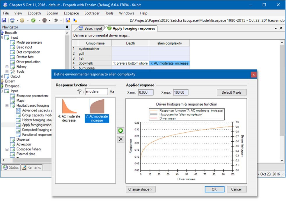
Make sure that sensitive groups are configured to derive foraging capacity from environmental drivers in Ecospace>Input>Habitat based foraging>Group capacity model.

When Ecospace next runs, this environmental driver will be used to help drive functional groups around the map, as dictated by the foraging capacity computed by the functional responses to ecosystem engineer‐computed structural complexity.

Make sure that sensitive groups are configured to derive foraging capacity from environmental drivers in Ecospace > Input > Habitat based foraging > Group capacity model (Figure 8).

When Ecospace next runs, this environmental driver will be used to help drive functional groups around the map, as dictated by the foraging capacity computed by the functional responses to ecosystem engineer‐computed structural complexity.

References

Concept: S. Sadchatheeswaran, Biological Sciences, University of Cape Town, South Africa

Coding: J. Steenbeek, Ecopath International Initiative, Spain

Financial contributions from the University of Cape Town, the Andrew Mellon Foundation, the South African Research Chair Initiative (funded through the South African Department of Science and Innovation (DSI) and administered by the South African National Research Foundation (NRF)), and the DSI‐NRF Centre of Excellence for Invasion Biology are gratefully acknowledged.