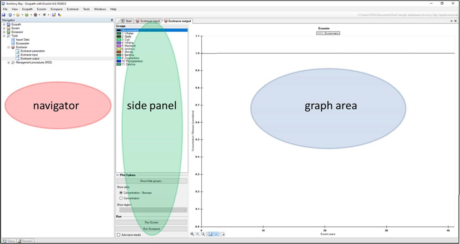
The interface for the output of the data involves the navigator, a side panel and a graph area (Figure 1). Ecotracer output is selected from the navigator to display the side panel and the graph area. Data on the side panel involves choosing the data that is to be displayed on the graph area, the type of contaminant data displayed, the data displayed on the graphing area, the specific routine run button, and whether or not the data is automatically saved. Once data has been entered into the input interface, the simulation is initiated from the output interface either through the Run Ecosim or Run Ecospace buttons on the side panel to the graphing interface.

The graphical interface displays how the contaminant in the environment and in each functional group changes through time. There is a choice between having the functional groups trace the contaminant by the amount (e.g., Bq) in the group or by the biomass concentration (e.g. Bq∙t‐1). The environmental concentration is essentially an area density (e.g., Bq∙km‐2). Under an assumption of environmental equilibrium, the environmental concentration on the graph should show a flat line. Under no changes to the functional groups underlying parameters (e.g., fishing mortality), the concentration in each group (e.g., Bq∙t‐1) should also be represented by a flat line.

For radioisotopes under assumed equilibrium conditions, the amount lost by radioactive decay would have to be added in as a base inflow rate to maintain equilibrium. Although equilibrium conditions may not be realistic, it is definitely a good way to see if the model is behaving properly, and may be a good assumption if the environmental concentrations do not change much due to a radioisotope having a long half‐life, or when long‐lived animals (e.g., whales) are not represented in the model as they would not be affected by historical environmental concentrations. The inverse of the P/B (unit: year-1) ratio is an indication of the average longevity of the groups in the model (B/P, unit: year).

Output files in Ecosim can be saved to a directory by selecting auto‐save results. In Ecospace, it is necessary to open Ecospace parameters on the navigator panel and then select the files under the auto‐save dialogue box. In most cases, the biomass maps and the contaminant concentration map need to be selected. This is because the concentration map is for the amount and therefore it is necessary to compute the concentration (e.g., Bq∙t‐1) from the two sets of data. The path directory for output files can be found in the status window. However, usually for the first run of a scenario it is useful to not save the data and examine the output by hovering over the concentration data on the graph; point‐values can be shown by right clicking on a line on the graph and selecting Show point values. After adjustments have been made to basic input parameters (Ecopath or Ecotracer) if required, and the point values are in the desired range of expected output values, it is then worthwhile to save the output files.

Currently post‐processing of the output files must be done in another program such as Microsoft Excel or R. Models that only use Ecosim for time dynamics will have a single output file containing a single column of output for each functional group, and 12 rows of data for each year with the cells containing the amount in the group. Models using Ecospace have CSV output files for each species that cover one time step for one species with the columns representing the longitudinal grid of the map and the rows the latitudinal grid working from the top left cell to the bottom right cell.

Changes in concentration for the environment and functional groups other than those resulting from changes in environmental concentrations result from the kinetic interactions as described earlier. Functional groups with no starting concentrations will have increasing concentrations, and groups with starting concentrations may have changes through time as a result of their losses and gains at each time step. However, differences between a functional group’s model output and those with a starting amount based on field collected samples can also be affected by biases in sampling (i.e., sampling not being representative of the population concerned) or by incorrect Ecopath or Ecotracer parameters. The biomass of a group may also change through time most commonly due to trophic interactions or changes in fishing mortalities if these are represented in the model. Thus, the resulting biomass concentrations can be a function of changes in the amount of contaminant in the functional groups and changes in the underlying state variables (biomass) through time.

Ecotracer is a useful computer simulation tool to gain knowledge on the transfer of pollutants in an ecosystem. We have attempted to give a practical guide to colleagues who are interested in the use of the EwE ecosystem modelling framework a better understanding on the technical use of the routine, and the interfaces used. We hope this inspires people from various backgrounds to engage and gain a better understanding of how contaminants behave in an ecosystem.

Attribution

This work has been funded by the Institut de Radioprotection et de Sûreté Nucléaire (IRSN) and the French program Investissement d’Avenir run by the National Research Agency (AMORAD project, grant ANR‐11‐RSNR‐0002, 2013‐2022).