Dispersal Rate IBM
Carl J. Walters and Villy Christensen
An Individual-Based Model and Utility for Estimating Diffusive Mixing Rates of Organisms Between Spatial Model Cells
Spatial models typically need to simulate diffusive spread of creatures between spatial model cells or grid points. We usually approximate this spread by estimating instantaneous movement rates between adjacent discrete model grid cells; in terms of mathematical diffusion theory, such rates are approximations for D/L2, where D (km2/time) is the theoretical diffusion coefficient for the diffusion process and L is the discrete cell length in km.
Instantaneous mixing rates for any particular creature depend on three factors: its swimming speed, how frequently it makes turns (changes in direction), and how much change in direction it is likely to make each time it turns. Mixing rates are predicted to increase with increasing swimming speed, but to decrease with increasing number of turns per day and increasing variability in the movement direction after each turn. There is no simple theoretical way to integrate these three effects into an instantaneous mixing rate estimate except under very restrictive assumptions about how the creature changes direction at each turn.
The Ecospace dispersal estimator Shiny app at Ecopath.app generates estimates of instantaneous mixing rates by the simple tactic of simulating movement over one day of a large number of individual fish that are initially distributed at random over one spatial model grid cell, while counting how many of these individuals cross the model cell boundary at least once over the day. The approximate instantaneous mixing rate per day is then just the number of fish that exit the cell divided by the number of fish simulated.
Swimming speed is typically predictable from body size (many organisms swim at about one body length per second for some proportion of each day), but the number of turns per day and how much direction changes at each turn may vary a lot depending in particular on how the creature searches for food, (e.g., whether it turns more frequently or tends to turn more sharply when it is in an area of high food concentration). Absent direct sample data on fine-scale movement patterns, you can at least obtain some range of credible estimates for the instantaneous daily mixing rate by varying the number of turns (or distance between turns), and how much variability there is from turn to turn in the change in direction.
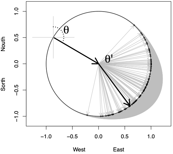
For each simulated movement step, each creature is assigned a random movement direction measured by the creature’s angle Ɵ in the X-Y plane (see Figure 1), and it moves a distance Dmove set by its movement speed and number of turns per day. Using a wrapped normal distribution, the movement angle Ɵ’ for its next move is set as Ɵ’=Ɵ+N(0,sd) where N(0,sd) is a normally distributed random deviate with mean 0 and standard deviation sd (radians). This method of generating random changes in direction results in creatures tending to keep going in the same direction if sd is small, (e.g., sd=0.2 [11˚ ]), and to make completely random direction changes at each move when sd is high, (e.g., sd=2 [115˚˚˚˚˚ ] For each model run, one of the individual movement patterns over the day is plotted, and model users are encouraged to do runs with multiple sd values so as to see the effect of the sd parameter on predicted movement trajectories. Note that similar results are obtained if there are many daily moves with low sd or fewer moves with high sd.
Note that estimates of instantaneous mixing rates from the IBM simulations can be badly biased downward for creatures that have high daily movement speed S, when the model cell length L is small compared to this speed, in particular if S/L is larger than about 0.5, (e.g., a tuna moving 80 km/day over a model grid of 20 km x 20 km cells has S/L=4). In such cases, the exit probability per day can approach 1.0. But the daily exit probability is only a good approximation for the daily instantaneous movement rate when this probability is very low, 0.05 or less.
Assumptions and Parameters
The utility is based on assumptions that,
- A swimming organism tends to move in a given direction with a swimming speed that is a function of its body length. Swim speed is usually a linear function of body length (bl). Typical numbers are 1 bl/sec when searching, 2 bl/sec when hunting actively, and 0.5 bl/sec when slowing down to feed. The swim speed is, however, species depending, and will be much lower for, e.g, ambush predators.
- Parameter: body length (cm).
- Parameter: CV of body length (Coefficient of Variation = standard deviation / mean)
- Parameter: swimming speed (body lengths per second).
- Parameter: CV of swimming speed
- The organism will change direction occasionally, notably after encountering potential prey and after being exposed to predators, so it will, e.g., be fewer turns per hour for a piscivore compared to a planktivore. How often does an organism make a turn? Run time is almost proportional to number of turns/hour.
- Parameter: number of turns per active hour
- Parameter: standard deviation of turns (in degrees)
- The organism is active for a number of hours each day. Some species may swim for 24 hours per day, with only ultra-brief micro sleeping episodes, others will build a cocoon and sleep the night away, and many are only active around dawn and dusk. Hence, the number of hours active per day is very species dependent. Run time is almost proportional to number of hours active per day.
- Parameter: number of hours active per day.
- Parameter: CV of number of hours active
- Some organisms may have a home base or range, and a propensity to stay near home
- Parameter: proportion of moves that are towards the home base or range
- Cell length, Ecospace does not keep track of where species are within cells, therefore the relationship between dispersal rate and cell size matters. The cell length parameter is easily available from the base map knowing the latitude and cell size. Use the average of cell height and cell width.
- Parameter: cell length (km)
- If cell size is small and swim speed is high, it may be necessary to simulate only a proportion of a day. The output is sensitive to this parameter setting.
- Parameter: Model simulation time (prop. of day)
- An IBM model, models, well individuals. By default the dispersal of 1000 individual organisms is simulated. This typically takes 1-2 seconds on the server (including transmission), so reasonably fast. Simulating more fish will take longer and not necessarily change the results.
- Parameter: Number of fish
- Simulation time: When exit probability > 0.05/day, we recommend you decrease the model simulation time. Default is one day.
- Parameter: Model simulation time (proportion of day)
The dispersal estimator IBM is implemented as a Shiny app at Ecopath.app‘s Dispersal IBM tab. and hosted at a site that hopefully will host also other Shiny apps [1] that may be of benefit for the Ecopath user community. Upon load of the app, it will let 1000 individual organisms (particles) move at random according for one day (24 hours) with the default parameter settings, and show the resulting Ecospace dispersal rates, a.o. Every time parameters are changed in the app it will redo the movements for the (by default) 1000 individual organisms, and it will store the input parameter settings along with the estimated parameters.
Action Buttons
Generate 20 runs: When clicked, will generate 20 random runs (each with however many organisms that is specified in the Number of fish setting. The results for the 20 runs are stored in memory, and can be saved with the Save session output button.
Save session output: By selecting the Save session output, the information from the entire session will be saved to a CSV file. If pressed consecutively, it will hold more and more information. The stored data will only be reset when the app is reloaded.
Output
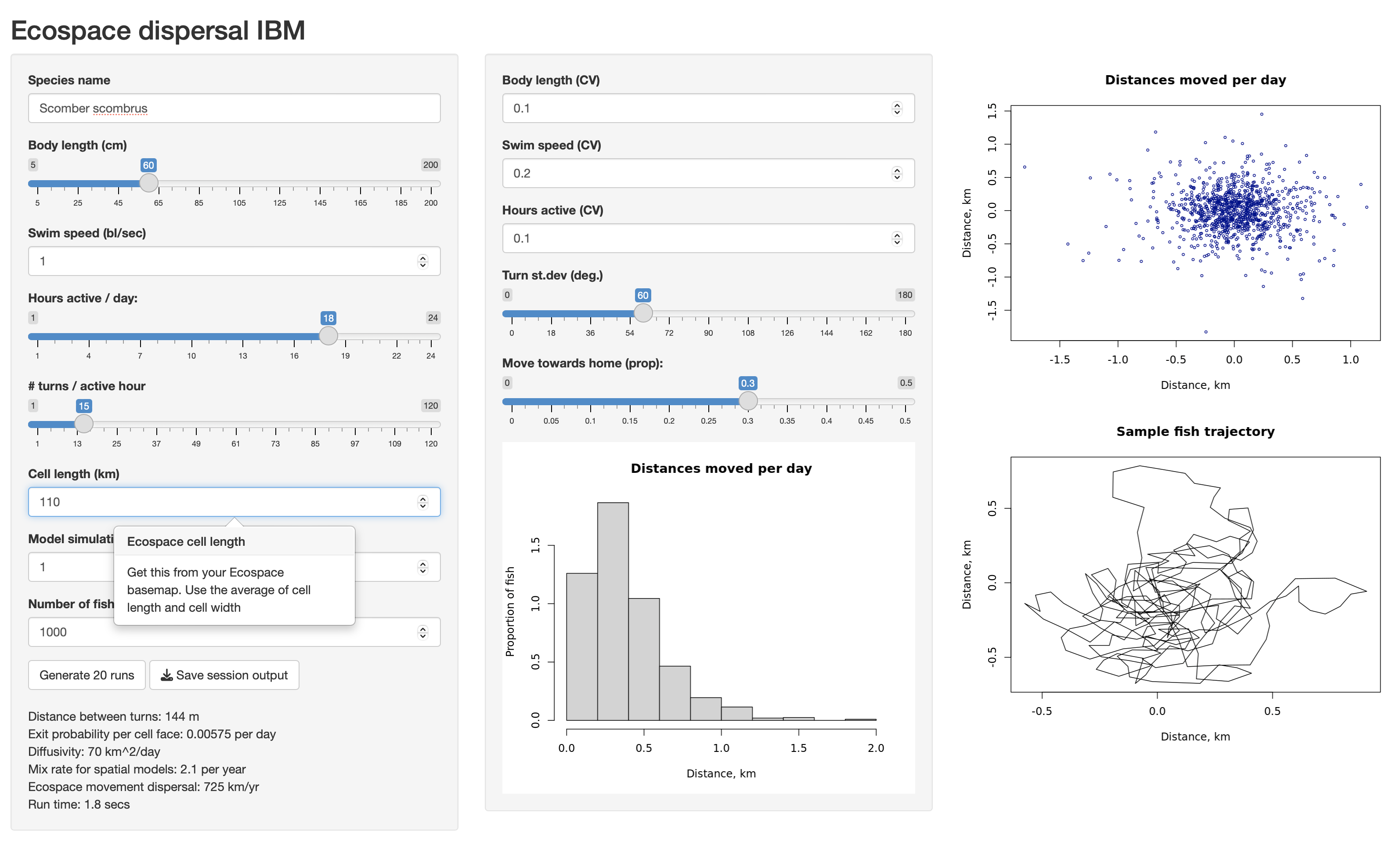
Distances moved per day (histogram, day-1): Estimated based on input parameter setting and averaged over the simulated number of fish (i.e. organisms) simulated.
Distances moved per day (scatter plot, day-1): Plot shows the distance moved during a day for each of the Number of fish organisms.
Sample fish trajectory (X-Y plot, day-1): The trajectory for the first organisms simulated, drawn with uncertainty in input parameters as represented based on the parameter uncertainty.
Distance between turns (m): Calculated as swim speed (bl/sec) x body length (cm) x 60 (sec/min) x 60 (min/hour) x 0.01 (m/cm).
Exit probability per cell face (per day): Calculated from average probability over each of the simulated number of organisms that they exit a cell within the time period simulated. When exit probability > 0.05/day, we recommend you decrease the model simulation time.
Diffusivity (km2/day): Calculated as exit probability / (cell length)2 / model steps per day
Mix rate for spatial models (year-1): Calculated as 365 x probability of exit / model steps per day
Ecospace movement dispersal (km year-1): Calculated as the mixing rate x cell length x π. This is the estimated dispersal rate for use in Ecospace.
Run time (secs): For information only, will provide some guidance for how long extended runs will take.
The Shiny R code for the dispersal simulator is available at this link.
- Let us know if you have an app that may be of interest ↵
