Driving Ecotracer with Spatial-Temporal Data
Shawn Booth; Jeroen Steenbeek; and Sabine Charmasson
Environmental distributions of contaminants can be made time‐varying through the spatial temporal framework (STDF). Incorporating monthly changing patterns of contaminant concentrations into Ecotracer is a three‐step process: 1) Prepare maps in a GIS; 2) define external data connections in EwE; and 3) connect an external data connection to drive the contents of the Ecospace contaminants layer.
Prepare Maps in a GIS
Although the STDF contains a GIS engine that converts GIS data to the Ecospace grid (Steenbeek et al. [1]), it is highly recommended that ecosystem modellers perform this step in a dedicated GIS software to minimize GIS processing artifacts.
The step to prepare maps in a GIS entails the necessary steps to convert contaminant distributions over time into discrete, monthly ESRI ASCII maps that match the exact dimensions, cell size, spatial extent, and geospatial projection of the base map in an Ecospace scenario.
The Ecospace base map can be extracted from a loaded Ecospace scenario as follows:
- Click Navigator > Ecospace > Input > Maps
- Double‐click the Depth layer at the right‐most panel
- In the Edit layer interface that appears, select the Data tab. In the Data tab, select Export > To ASCII…
The actual steps to convert contaminant distributions to monthly Ecospace maps can require a number of GIS operations, depending on the format and content of the original contaminant data. Operations may require:
- Reprojecting to the Ecospace base map (most likely WGS84 / epsg:4326)
- Temporal clustering
- Clipping
- Kriging (point data) and/or resampling (vector data)
- Exporting to the ESRI ASCII format.
Define External Data Connections in EwE
Once one or more time series of monthly ASCII maps have been prepared, Ecospace needs to know where to find these time series on the local machine. Do the following,
- Click Menu > Ecospace > Define external data connections…
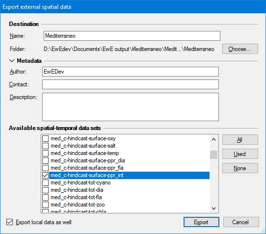
Figure 1 – To define a new spatial‐temporal data connection, select the type of the connection and click . From this interface one can also reconfigure external data connections that were previously created. - In the Define external data connections interface, select connection type A series of Ecospace ASCII maps over time and click Create (Figure 1). This will define the time series, and will bring up the Configure external data interface to configure the new time series (Figure 2).
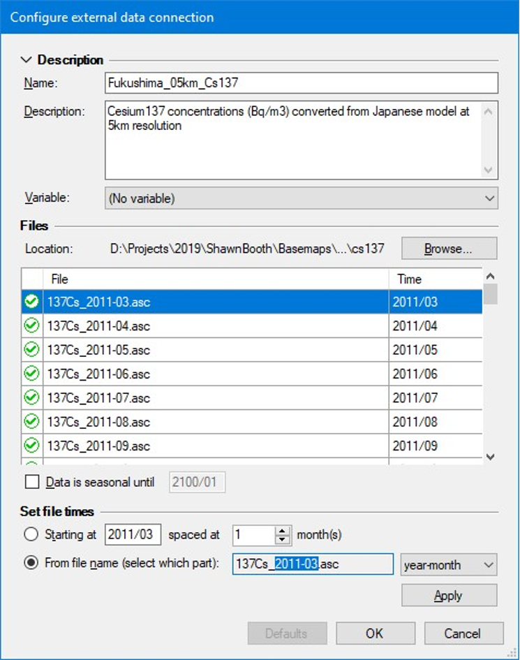
Figure 2 – The interface to configure a specific external data connection (e.g, a time series of maps). Each time series has a name to uniquely define the series in the Ecopath with Ecosim user interface, an optional description, a variable that only serves to limit where the external data connection appears in the Ecopath with Ecosim user interface, and a series of timetagged maps that, in this particular figure, reflects historical concentrations of 137Cs in the water off of Fukushima, at monthly time steps, since March 2011. - In the Configure external data interface, enter a unique name to identify the time series in the Ecopath with Ecosim user interface.
- It is advisable to use the description to describe where the maps time series came from.
- The variable field serves to limit where the external data connection appears in the EwE user interface. For contaminants, leave this field at its default value (No variable).
- Now add the actual maps to the external data connection. Click Browse and navigate the folder that contains the maps. Select all the maps, and click Open. The maps will appear in the Configure external data interface.
- This interface has limited abilities to parse the date from map file names. Please check the Time column and ensure that each map has a correct time tag. You can modify time tags by hand, or with the tools provided in the Set file times section.
- Once all maps are correctly time‐tagged, close the Configure external data. The newly configured time series of external maps will appear in the Define external data connections interface.
- Close this interface too.
Ecospace now has the information to locate and integrate time series of external ASCII contaminant maps into the running model.
Connect the External Data to the Contaminants Layer
Now at least one time series of contaminants in seawater has been defined, this time series needs to be connected to drive the contents of the Ecospace contaminants map layer. Do the following,
- In the Navigator, open Ecospace > Input > External data (Figure 3)
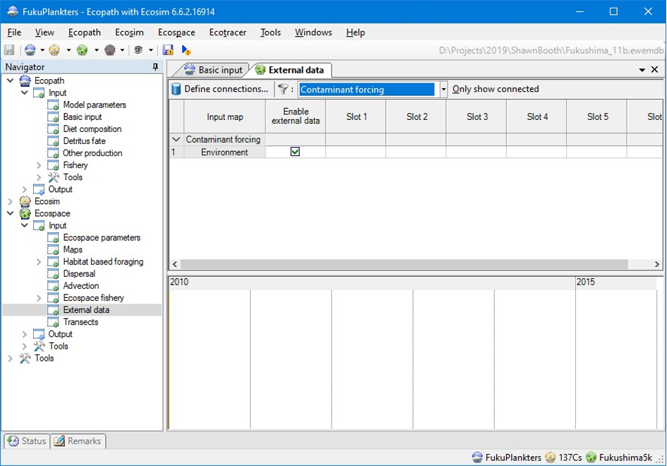
Figure 3 – The External data interface where previously defined external data connections are applied to Ecospace layers. - Under input maps, locate the environmental contaminants map. One can also use the on‐screen filter options to reduce the number of visible input maps
- In the row for the environmental contaminants map, click the cell Slot 1 to assign an external connection here. This brings up an interface dedicated to configuring how external data is integrated into Ecospace (Figure 4)
Figure 4 – Configuring the integration of an external time series of maps into Ecospace, in this case to the environmental contaminants layer. Applied external time series are shown as “Connected”. The selected connection can be configured, which includes entering a scaling factor to ensure that external data matches the magnitude of data currently in the Ecospace environmental contaminants layer. As described in Steenbeek et al., the Calculate option scales the average map mean for the first full year of external data to the map data loaded in Ecospace. - Here, from the list of available connections, select the connection that you wish to apply, and click the Apply (green arrow pointing right) button. The connection now appears under the list of Connected external data connections.
- An important aspect is to set a proper scale to ensure that the tracer (e.g., 137Cs) concentrations as obtained from external data is properly scaled to the units expected by Ecospace.
- Click Close.
- Run Ecospace.
Attribution
This work has been funded by the Institut de Radioprotection et de Sûreté Nucléaire (IRSN) and the French program Investissement d’Avenir run by the National Research Agency (AMORAD project, grant ANR‐11‐RSNR‐0002, 2013‐2022).
- Steenbeek, J., Coll, M., Gurney, L., Mélin, F., Hoepffner, N., Buszowski, J., Christensen, V., 2013. Bridging the gap between ecosystem modeling tools and geographic information systems: Driving a food web model with external spatial–temporal data. Ecological Modelling 263, 139–151. https://doi.org/10.1016/j.ecolmodel.2013.04.027 ↵
