It’s a fascinating aspect of food web models that one can deduct quite a bit about the ecosystem form and functioning simply from the flows and state variables in the food web, from the ecosystem flow chart.  This is different though from what can be deducted from a more complex dynamic model. You could think of it as the difference between analyzing a single picture and watching a movie. It’s different things, different questions, all with their value. The value of the food web representation comes from it being simple, well rather simple, it can be complex or messy given enough functional groups. But there are lessons to be drawn from such simple representations.

To get to those lessons, we need indicators. The food web per se is indeed quite messy to examine, and we use indicators to make sense of such messiness.  The field of network analysis is built around this, what can one deduct from a network such as represented by a food web?  EwE to that effect has a network analysis plug-in with the more complex analysis, while a suite of indicators are given in the Ecopath > Output forms, which is the topic of this chapter.

Once you have entered sufficient input parameters, you can proceed to the output forms where on the Ecopath > Output > Basic estimates form, the missing parameters will be estimated so that mass balance is achieved. Both input (black font) and calculated (blue font) parameters are displayed.

If Ecopath has NOT been balanced already since opening or making changes to the input parameters, selecting any of the output forms will cause Ecopath to attempt to balance the model. Note also that you will not be able to balance your model if the sum of the diet composition for each consumer group does not sum to 1. Return to the Ecopath > Input > Diet composition form and fix the problem if this is the case.When you create an Ecopath model and need to mass-balance it, know that uncertainty can be dealt with later. To get started, we need a plausible model, not the correct model (which doesn’t exist) but one that can be used for, e.g., making thousands of models based on parameter uncertainty.

Problems in parameter estimation will be shown in the Status panel. Two types of message may be displayed in the Status panel while you are balancing your model

• Information messages provide feedback on regular events in EwE. Information events are confirmations of things that went well. Examples are opening the model; successful edits; and successful balancing (i.e., parameterization) of the model.
• Warning messages when EwE was not able to complete an action and requires the user to fix a problem, usually with the input data. For example, one of the most important of these is when parameterization fails (i..e., the model failed to balance). When this occurs, you will get the message “Your model is NOT balanced! Computed Ecotrophic Efficiencies (EE) invalid for one or more group(s).” Clicking on the “+” icon next to this message expands the message to show which groups are causing the problem.

Basic Estimates

Most of the parameters on this screen are input values and therefore discussed in that section of this guide.

Trophic Level

Lindeman ^[1] introduced the concept of trophic levels. In Ecopath, the trophic levels are not necessarily integers (1, 2, 3…) as proposed by Lindeman, but can be fractional (e.g., 1.3, 2.7, etc.) as introduced by Odum and Heald ^[2]. A routine assigns definitional trophic levels (TL) of 1 to producers and detritus and a trophic level of 1 + [the weighted average of the preys’ trophic level] to consumers.

Following this approach, a consumer eating 40% plants (with TL = 1) and 60% herbivores (with TL = 2) will have a trophic level of 1 + [0.4 · 1 + 0.6 · 2] = 2.6. The fishery is assigned a trophic level corresponding to the average trophic level of the catch, i.e. without adding 1 as is done for ‘ordinary’ predators.

The trophic level is a dimensionless index.

Key Indices

Net Migration

The net migration, E,  is calculated as emigration less immigration. This means that net migration will be negative if there is more coming into the system than leaving it, i.e. it will be a negative production term, which perhaps may balance a higher fishing mortality or an increase in biomass accumulation.

Flow to Detritus (FlowToDet)

For each group, the flow to the detritus consists of what is egested or excreted (the non-assimilated food) and those elements of the group that die of old age, diseases, etc., (i.e., of sources of ‘other mortality’, expressed by 1 – EE). The flow to the detritus, expressed, e.g., in t km^-2 year^-1, should be positive for all groups.

Net Efficiency

The net food conversion efficiency is calculated as the production divided by the assimilated part of the food, i.e.,

Net efficiency = P/B / (Q/B · (1 – U))

where P/B is the production / biomass ratio, Q/B is the consumption / biomass ratio, and U is the proportion of the food that is not assimilated (but egested or excreted).

The net efficiency can also be expressed,

Net efficiency = production / (production + respiration)

The net efficiency is a dimensionless fraction. It is positive and, in nearly all cases, less than 1, the exceptions being groups with intermediate trophic modes, e.g., groups with symbiotic algae. The net efficiency cannot be lower than the gross food conversion efficiency, g.

Omnivory Index

The ‘omnivory index’ was introduced in 1987 (Pauly et al., 1993a) in the initial, unreleased version of the Ecopath II software. This index (OI_j) is calculated as the variance of the trophic level of a consumer’s (j) prey groups (i). Thus

[latex]OI_j = \sum \limits_{i=1}^{n}(TL_i-(TL_j-1))^2 \cdot DC_{ji} \tag{1}[/latex]

where, TL_i is the trophic level of prey i, TL_j is the trophic level of the predator j, and, DC_ji is the proportion prey i constitutes to the diet of predator j.

When the value of the omnivory index is zero, the consumer in question is specialized, i.e., it feeds on a single trophic level. A large value indicates that the consumer feeds on many trophic levels. The omnivory index is dimensionless.

The square root of the omnivory index is the standard error of the trophic level, and a measure of the uncertainty about its precise value due to both omnivory and sampling variability.

Mortality Rates

The three forms in this node are arguably the most important reference for the user during the model-balancing process, as they can be used to indicate which mortality components are most likely to be causing problems.

Mortalities

The mortality coefficients form (Figure 1) is one of the most important forms on the Parameterization menu and it is, as a rule, the first that should be checked when balancing a model.

Components of Mortality in Ecopath

Under equilibrium assumptions, each group can be represented by an average organism, with an average weight. This makes it possible to use equations for estimating mortality in numbers, even when dealing with biomass. One such equation is[latex]N_t=N_0 \cdot e^{-Zt}[/latex] where N₀ is a number of organism at time 0; N_t is the number of survivors at time t; and Z is the instantaneous rate of mortality (year^-1).

Under the assumption that Z_i, the mortality of group i, is constant for the organisms included in i it turns out that for a large number of growth functions (including the von Bertalanffy Growth Function, or VBGF)

[latex]Z_i=(production / biomass)_i= (P/B)_i \tag{2}[/latex]

or instantaneous mortality equals total production over mean biomass ^[3].

The mortality coefficient can be split into its components following a well-known procedure, i.e., the second Ecopath Master Equation,

Z_i = (P/B)_i = Fishing mortality + Predation mortality + Biomass accumulation + Net migration + Other mortality

or

[latex]Z_i = (P/B)_i = F_i+M2_i+BA_i+E_i+M0_i \tag{3}[/latex]

Where for group I,

• F_i is the fishing mortality rate;
• M2_i is the predation mortality rate;
• BA_i is the biomass accumulation rate (actually BA_i/B_i);
• E_i is the net migration rate (emigration less immigration).M0_i is the other mortality rate.

All are with the unit year^-1 as they are rates (t km^-2 year^-1) relative to biomass (t km^-2).

In some models, (notably the Multispecies Virtual Population Analysis), the ‘other mortality’ component is split between M1, i.e., predation by predators not included in the model, and M0, ‘other mortality’, caused by diseases, senescence, etc. In Ecopath, M1 is included in M0, as models often are intended to describe the major components of predation mortality explicitly (so M1 is likely to be minimal). Further, M0 is not entered directly, but is computed from the ecotrophic efficiency, EE.

Ecopath-predicted values for these coefficients are given on the Mortality coefficients form. The mortality coefficients are estimated from the following equations:

[latex]Z_i = (P/B)_i\tag{4}[/latex]

[latex]M2_i=\sum\limits_i B_i \cdot(Q/B)_i \cdot DC_{ji}/Bi\tag{5}[/latex]

[latex]F_i = C_i/B_i\tag{6}[/latex]

[latex]M0_i=(1-EE_i)\cdot (P/B)_i\tag{7}[/latex]

where (Q/B)_j is the consumption/biomass ratio of predator j; DC_ji is the proportion prey i contributes to the diet of predator j, B_i is the average biomass of i, and C_i is the catch of i. The biomass accumulation term, BA_i, is a basic input term.

Predation Mortality

The predation mortality of a group i is the sum of the consumption of i by all groups (including i), divided by the biomass of group i. Predation mortality is calculated from (7), i.e., it is not an input parameter.

When you balance a model, and you have a group that does not balance (EE >1), the first thing to do is to check the Ecopath > Output > Mortality rates > Mortalities form (as described above in this chapter) to evaluate if the problem is due to fishing or predation (one of which or both often being the culprit). If it is due to predation, the next step is to check the Ecopath > Output > Mortality rates > Predation mortality rates form (Figure 8).

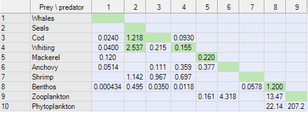
The form will guide you to particular mortality coefficients that are causing problems with balancing. If predation mortality is too high then the form will help you identify which predators that are causing the problem for a particular prey group.

To help you identify possible problem predators, cells with unusually high predation mortalities will be shown with a different-coloured background instead of the usual background (as is the case for seals predation on cod and whiting in Figure 1).

Consumption

The Ecopath estimates of consumption (food intake) can be found at Ecopath > Output > Consumption. The consumption of a living group is the product of its biomass (B) times its consumption/biomass ratio (Q/B). The food intake is a flow rate expressed, e.g., as t km^-2 year^-1.

The consumption table also displays all flows to the detritus group(s) even though it is not consumption, (we had to put it somewhere).

Respiration

The Ecopath estimates of respiration are at Ecopath > Output > Respiration. The Respiration form displays the predicted values for respiration and assimilation of food by all groups.

Respiration

Respiration includes all non-usable ‘model currency’ that leaves the box representing a group.

When the currency is energy or carbon, the bulk of the assimilated food will end up as respiration. If, however, a nutrient (e.g. phosphorus or nitrogen) is used as currency, all nutrients that leave the box is re-utilized; in this case, respiration is nil.

Primary producers will not have respiration if the unit is energy based.

Since assimilated food ends up as either production or respiration, only one of these two quantities needs to be estimated, as the other – here respiration – can be calculated as a difference. In Ecopath, this is calculated as the difference between the assimilated part of the consumption and that part of production that is not attributable to primary production (i.e., 1 – TM). Thus, for groups with intermediate values of TM, i.e., for mixed producers/consumers, only that part of the production that is not attributable to primary production is subtracted. For reasons of consistency, in Ecopath, detritus is assumed not to respire, although it would if bacteria were considered part of the detritus, (which is one reason why it is better to create one or more separate groups for the detritus-feeding bacteria if this difficult group is to be considered at all).

The respiration of any living group (i) can be expressed as,

[latex]Resp_i = (1-U_i) \cdot Q_i - (1-TM_i)\cdot P_i \tag{8}[/latex]

where Resp_i is the respiration of group i, U_i is the fraction of i‘s consumption that is not assimilated, Q_i is the consumption of i, and TM_i is the proportion of the production that can be attributed to primary production. If the unit is a nutrient, TM_i is equal to zero, irrespective of whether the group is an autotroph or not (nutrients are not produced), and, P_i is the total production of group i.

Respiration is used, in Ecopath, only for balancing the flows between groups. Thus, it is not possible to enter respiration data. However, known respiration values (i.e., the metabolic rate) of a group can be compared with the output, and the input parameters adjusted to achieve the desired respiration.

Respiration is a non-negative flow expressed, e.g., in t km^-2 year^-1. If the currency is a nutrient, (e.g., nitrogen or phosphorus), respiration is zero: nutrients are not respired, but egested or excreted and recycled within systems.

Assimilation

The part of the food intake that is assimilated is computed for each consumer group from

[latex]B_i \cdot (Q/B)_i \cdot (1-U_i) \tag{9}[/latex]

where B_i is the biomass of group i; (Q/B)_i is the consumption / biomass ratio of group i; and U_i is the part of the consumption that is not assimilated.

The three parameters needed for the estimation are all input parameters. Assimilation is a flow expressed, e.g., in t km^-2 year^-1.

Respiration/Assimilation

The (dimensionless) ratio of respiration to assimilation cannot exceed 1 as respiration cannot exceed assimilation. For top predators, whose production is relatively low, the respiration/assimilation ratio can be expected to be close to 1, while it will tend to be lower, but still positive, for organisms at lower trophic levels.

Production/Respiration

The (dimensionless) ratio production / respiration express the fate of the assimilated food. Computationally, this ratio can take any positive value, though thermodynamic constraints limit the realized range of this ratio to values lower than 1.

Respiration/Biomass

The R/B ratio can be seen as an expression of the activity of the group. The higher the activity-level is for a given group, the higher the ratio. The R/B ratio is strongly impacted by the assumed fraction of the food that is not assimilated, see the basic input form. If the ratio is too high, this may be due to GS being too low. The R/B ratio may be available in the physiological literature for  some species/groups.

The ratio respiration / biomass can take any positive value, and has the dimension year^-1.

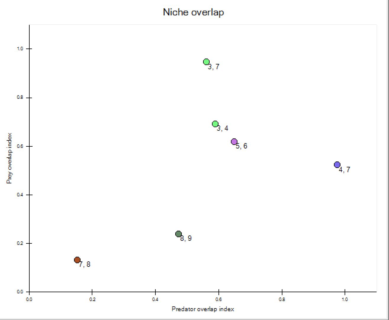
Niche Overlap

Niche overlap indices for Ecopath models are available at three Ecopath > Output > Niche overlap forms

For this, a simple niche overlap index is adopted, and it is shown how it can serve as a starting point for the development of a new (predator) niche overlap index incorporating predation. The procedure involved in deriving a predator niche overlap index (from a prey niche overlap index) should be generally applicable, i.e., not limited to the type of index presented below.

Pianka (1973) suggested the use of an overlap index derived from the competition coefficients of the Lotka-Volterra equations. This index, O_jk, which has been used for many descriptions of niche overlap, can be estimated, for two species/groups j and k, from

[latex]O_{jk} = \sum\limits_{i=1}^{n}(p_{ji}\cdot p_{ki})/\sqrt{\sum \limits_{i=1}^{n}p_{ji}^2 \cdot p_{ki}^2}\tag{10}[/latex]

where P_ji and P_ki are the proportions of the resource i used by species j and k, respectively. The index is symmetrical and assumes values between 0 and 1. A value of 0 suggests that the two species do not share resources, 1 indicates complete overlap, and intermediate values show partial overlap in resource utilization.

Closer examination of the Pianka overlap index shows it to have an unwanted characteristic and it is therefore slightly modified here. If one of the groups (say j) only overlaps with one other group k then P_ji will be zero for all values of i but i = k, where it will reach a value of 1. In such a case, the denominator of (12) will always be 1, and the overlap index will equal P_ki, whereas a value between P_ki and P_ji would be more reasonable. This behaviour is caused by the geometric mean implied in the denominator of (12) , and can be circumvented by the use of an arithmetic mean. For this, (12) is changed to

[latex]O_{jk} = \sum\limits_{i=1}^{n}(p_{ji}\cdot p_{ki})/\sqrt{\sum \limits_{i=1}^{n}p_{ji}^2 + p_{ki}^2}\tag{11}[/latex]

where the index and all of its terms can be interpreted as above. This version of the Pianka overlap index is used subsequently.

The niche overlap index can be used to describe various kinds of niche partitioning. Here attention will be focused on the trophic aspects. In this case, the P_ki and P_ji in (13) can be interpreted as the fraction prey i contributes to the diets of j and k, respectively.

Using an approach similar to that above, it is possible to quantify the predation on all preys m and n by all predators l, and to derive a ‘predator’ composition, estimated from

[latex]\bar X_{ml}=Q_iP_{lm}/\sum\limits_{l=1}^{n}(Q_l\cdot P_{lm}) \tag{12}[/latex]

and

[latex]\bar X_{nl}=Q_iP_{ln}/\sum\limits_{l=1}^{n}(Q_l\cdot P_{ln}) \tag{13}[/latex]

Here [latex]\bar X_{nl}[/latex]Xml can be interpreted as the fraction the predation by l contributes to the total predation on m, while Q_l is the total consumption for predator l. The predator compositions given above correspond to what Augoustinovics ^[4] defined, in the context of input-output analysis, as ‘technical coefficients’.

Based on the predator composition a ‘predator overlap index’ (P) can be derived as

[latex]P_{mn}=\sum \limits_{l=1}^{n}(\bar X_{ml}\cdot \bar X_{nl})/(\sum\limits_{l=1}^{n}(x_{ml}^2+x_{nl}^2)/2)\tag{14}[/latex]

the values of this predator overlap index range between 0 and 1 and can be interpreted in the same way as those of the prey overlap index, given in (13) .

In the present version, only one type of niche overlap index is incorporated, but both predator and prey niche overlap is given for this index. If of interest, more indices may be included in upcoming versions of EwE.

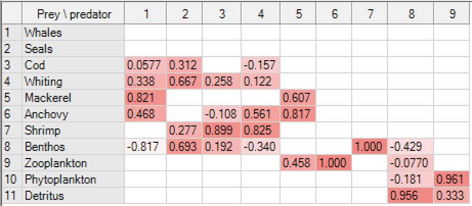
Electivity

The electivity (selection index) describe a predator’s preference for prey. It scales from -1 to 1; where -1 indicates total avoidance of a prey; 0 indicates that a prey is taken in proportion to its abundance in the ecosystem; and 1 indicates total preference for a prey. The electivity values are highlighted using a colour scale for the background, scaling from –1 (white) to 1 (red) using shades of red for intermediate values. The electivity index displayed is the standardized forage ration of Chesson ^[5](1983), see below.

One of the most widely used indices for selection is the Ivlev electivity index, E_i ^[6] defined for a group i as:

[latex]E_i=(r_i-P_i)/(r_i+P_i)\tag{15}[/latex]

where r_i is the relative abundance of a prey in a predator’s diet and P_i is the prey’s relative abundance in the ecosystem. E_i is scaled so that E_i = -1 corresponds to total avoidance of, E_i = 0 represents non-selective feeding on, and E_i = 1 shows exclusive feeding on a given prey i. Note that within Ecopath, r_i and P_i refer to biomass, not numbers.

The Ivlev electivity index while widely used has a major shortcoming, seriously limiting its usefulness as a selection index, it is not independent of prey density. A more versatile approach is to use the standardized forage ratio (S_i) as suggested by Chesson ^[7]. This index is independent of prey availability, and is given by

[latex]S_i=\frac{r_i/P_i}{\sum\limits_{j=1}^{n}r_j/P_j}\tag{16}[/latex]

where r_i and Pi are defined as above, and n is the number of groups in the system. The standardized forage ratio as originally presented takes values between 0 and 1, with Si = 0 representing avoidance and Si = 1 exclusive feeding. As implemented in EwE, the forage ratio has been transformed (linearly) such as to vary between -1 and 1, so that -1, 0 and 1 can be interpreted as for the Ivlev index.

Search Rates

A useful feature of the system of linear equations underlying the Ecopath approach (link) is that it can be used to estimate the Lotka-Volterra mass-action term a, which has the dimension of a volume searched per unit time by a given predator j seeking a certain prey i. Building on the second Ecopath Master Equation

[latex]B_i \cdot (P/B)_i \cdot EE_i - \sum\limits_{j}B_j\cdot (Q/B)_j \cdot DC_{ji}-C_i-E_i-BA_i = 0 \tag{17}[/latex]

where B is biomass, P production rate, EE the ecotrophic efficiency, C the catch rate, BA the biomass accumulation rate, E the net migration rate, Q the consumption rate, DC_ji the proportion i contributes to the diet of j (each of the consumers). Separating the biomass accumulation rate, BA, and re-expressing as a differential equation

[latex]BA_i=\frac{dB}{dt}=B_i\cdot (P/B)_i \cdot EE_i -\sum\limits_{j}B_j\cdot (Q/B)_j\cdot DC_{ji}-C_i-E_i = \ ... \ = B_i \cdot (P/B)_i \cdot EE_i - C_i - E_i-\sum\limits_{j}Q_{ji}\tag{18}[/latex]

where Q_ji expresses the consumption rate for consumer j of prey i. We can then solve for a_ji = Q_ji/(B_j B_i), which defines the Lotka-Volterra mass-action term a as the quotient of the amount of i consumed by j, divided by the product of their biomasses.

This mass-action term is a proportionality factor used in Ecosim to estimate consumption rate for consumers, given the changing biomasses of their preys, and their own changing biomasses.

The values of a depend obviously on the units used, and the biomass units used in Ecopath render difficult a direct interpretation of the numbers in the Ecopath > Output > Search rates table. However, they can easily be converted into values of a applying to single organisms, given that the ratio of the individual prey and predator weights are divided into the values of a for each pair of prey and predator.

Fishery

The Ecopath > Output > Fishery > Catch form and Ecopath > Output > Fishery > Value form summarizes total catch by quantity and value for each fished group by fleet. In connection with the EU Landing Obligation regulations, considerable capacity to handle discard dynamics have been added to EwE, and part of this are presented in the Ecopath > Output > Fishery > Discard mortality, Ecopath > Output > Fishery > Discard survival and Ecopath > Output > Fishery > Computed landings forms.

Catch

The Ecopath < Output < Fishery > Catch from shows total catch for fished groups by fleet, where

Catch = Landings + Discards

where landings and discards are entered as inputs at the Ecopath < Input < Fishery > Landings and Discards forms, respectively. The form also displays the trophic level of each fleet and of the fishery in total. For this, the trophic level is calculated similarly to how the trophic level is calculated for functional groups – as the average trophic level of the catch + 1.

Value

The Value form shows the calculated value for fished groups (i) by fleet (g), where

Value_i,g = Market price_i,g x Landings_i,g

where market price and landings are input from the Ecopath < Input < Fishery > Off-vessel price and Ecopath < Input < Fishery > Landings forms, respectively. The market value is with unit monetary value per year.

The non-market value of each resource is also shown in a separate column on the Ecopath > Output > Fishery > Value form (if any non-market prices have been defined on the Ecopath > Input > Fishery > Non-market value form. The non-market value is calculated for group i as

Non-market value_i = Non-market price_i x Biomass_i

The non-market value is with unit monetary value per year.

Discard Mortality

Discard mortality is at the Ecopath > Output > Fishery > Discard mortality form and is for group i caught by fleet g calculated as,

Discard mortality_i,g = Discard_i,g x Discard mortality rate_i,g

where the discard and discard mortality rate is obtained from Ecopath < Input < Fishery > Discards and Ecopath < Input < Fishery > Discard mortality rate respectively. Discard mortality is a flow rate with unit t km^-2 year^-1.

Discard Survival

Discard survival is at the Ecopath > Output > Fishery > Discard survival form and is for group i caught by fleet g calculated as,

Discard mortality_i,g = Discard_i,g x (1 – Discard mortality rate_i,g)

where the discard and discard mortality rate is obtained from Ecopath < Input < Fishery > Discards and Ecopath < Input < Fishery > Discard mortality rate respectively. Discard survival is a flow rate with unit t km^-2 year^-1.

Computed Landings

The computed landings at the Ecopath > Output > Fishery > Computed landings form should correspond closely to the input landings at the Ecopath > Input > Fishery > Landings form and I am not sure why the computed landings have been added. The computed landings are flow rates with unit unit t km^-2 year^-1.

Particle size distribution

later gator – REMOVE?