Ecotracer is a useful tool within the Ecopath and Ecosim (EwE) modelling approach to track radioisotopes, contaminants, persistent pollutants, or stable isotopes through a food web model.  After achieving a mass‐balanced Ecopath model, Ecotracer can be used with the Ecosim (time dynamic) or Ecospace (spatial‐temporal dynamic) to track the flow of the pollutant through the modelled ecosystem.

EwE uses a mass‐balance approach, and the flows of a contaminant due to predator/prey interactions are tracked within the underlying Ecopath model. However, Ecotracer also needs parameters for groups based on a kinetic toxicology approach to estimate initial conditions. However, similar to Ecopath, Ecotracer can become dynamic through either the use of Ecosim or Ecospace to follow the changes of a contaminant that has different temporal inputs or to variations in temporal spatial concentrations in the water column.

The Ecotracer interface involves a number of input parameters (e.g., BI) and some that are calculated internally by the program, (e.g., gains from diet). Ecotracer’s interface can be loaded from the task bar or from the side‐menu. The interface is divided into three parts: the side panel (navigator) to choose Ecotracer or one of the other components of EwE; the interface for input for the environment; and input data for the functional groups based on the Ecopath model (Figure 1). The fields for the environment and the functional groups, their description and units are described below.

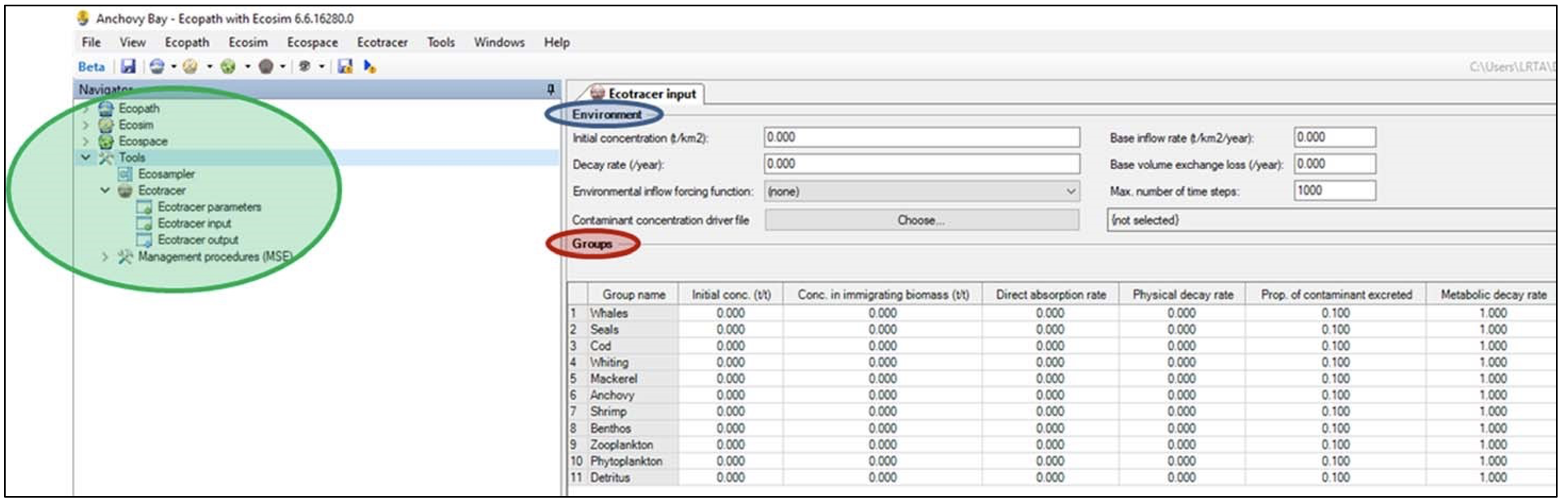
Navigator

The side panel allows easy access to the different routines within the EwE modelling framework. After creating a balanced Ecopath model, the Ecotracer routine can be selected in this area. Ecotracer parameters must be selected and a name can be given to the scenario. Also, it is necessary to select either ‘enable contaminant tracing for Ecosim’ if the model is only being run forward in time or ‘enable contaminant tracing for Ecospace’ if the model is spatialized using the Ecospace. The selection of which is dependent upon the underlying model and whether there are time or spatial‐temporal dynamics that are of interest.

Troubleshooting: if you do not get a response in Ecotracer and you have entered a direct absorption rate for primary producers; ensure that Ecosim or Ecospace have the contaminant tracing box checked.

Environment

The simplest case for the environment is if the model area has a near uniform concentration. If this is the case then one concentration can be used for the initial concentration of the environment. If there are differences in time, but the spatial area is treated as being homogenous in concentration, then the base inflow rate can be changed using a csv file that represents either absolute or relative changes to the initial environmental concentration. If there are spatial‐temporal variations in environmental contaminants in the model area, then a professional license for EwE is needed. Through the Spatial Temporal Data Framework (STDF ^[1], see chapter Spatial‐Temporal Data Framework), monthly maps of contaminant concentrations can be inserted into Ecotracer, enabling modellers to incorporate historical and/or projected environmental contaminants into Ecotracer. Brief instructions how to use the STDF with Ecotracer are provided as an annex at the end of this manual.

Initial concentration: concentration in the water. Currently, there is no explicit depth representation in Ecospace and to be consistent with the biomass units (i.e., t∙km‐2) in Ecopath the units are expressed per km2 with the units commonly being mass for most contaminants (e.g., g∙km‐2) or becquerels for radioisotopes (i.e., Bq∙km‐2). Therefore, units expressed in terms of unit per volume (e.g., μg∙L‐1) must be converted to the spatial resolution used.

Base inflow rate: the amount entering the environment each year (e.g., g∙km‐2∙year‐1). Obviously a base inflow rate for a one time release of, for instance, a hazardous chemical would not need a base inflow rate. However, to maintain background levels under equilibrium conditions a base inflow rate is needed to account for uptake and/or physical decay rates of the contaminant.

Base volume exchange loss: the rate at which a contaminant is lost to the environment (year‐1).

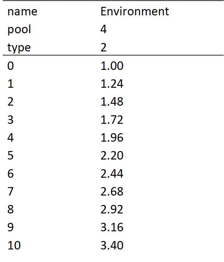
File for Base Inflow Rate: this is intended to be used when the environment receives a uniform increase. This is a .csv file that is arranged to implement changes to the environment on a relative or absolute scale through time (Table 1).

Table 1: Environmental inflow forcing function file that changes the relative base inflow rate from 1 to 3.40 over ten years; pool indicates the environment; and type 2 signifies a relative rate to the original environmental concentrations.

File for Point source Release: the point source release is another way of implementing changes to the environment on a spatial‐temporal scale in conjunction with Ecospace. It requires a series of ASCII files to implement the changes in a spatial cell through time and is a feature of the EwE pro license.

Maximum number of time steps: Ecotracer numerically solves the equations at a higher resolution (i.e., more time steps) than Ecopath, Ecosim and Ecospace, which all have monthly time steps in order to reach a stable solution using an explicit integration method. The number of time steps is important for some contaminants that have relatively high physical decay rates. Therefore, the time steps and the number of calculations are increased to accurately trace the contaminant within Ecotracer, but Ecotracer integrates itself with the monthly time steps of Ecopath, Ecosim and Ecospace.

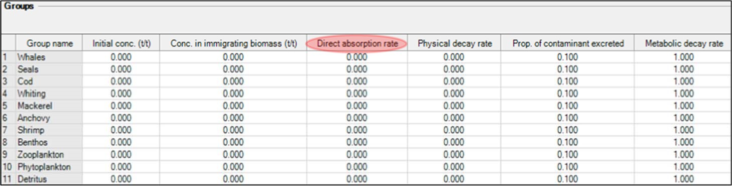
Biota

For ease of computation within the Ecotracer program, Ecotracer uses the amount of substance (e.g., Bq or g). However, for output (see next chapter) you can choose between the amount in a group (e.g., Bq) or biomass concentration (e.g., g∙t‐1). When validating model output to field sample data, it is likely that you will be comparing the biomass concentrations. All functional groups do not need to have starting concentrations, but they should have estimates of direct uptake rates, otherwise the resulting biomass concentrations will only reflect dietary uptakes based on the diet compositions entered for the Ecopath model. While this may not be important for top piscivores due to the fact that their diets mostly determine their contaminant load, it may affect the lower trophic levels of the food web where direct uptake rates may be more important than diet, and are the only entry way for primary producers. Dietary uptake is not entered as part of the Ecotracer routine as it is determined from the diet matrix, the consumption rate, the unassimilated amount, and the proportion of contaminant excreted.

Initial conc: the amount (e.g., Bq) in a group at the start of the model period (i.e., t = 0). Groups with no data from sample surveys can have a starting amount of zero.

Concentration in immigrating biomass: the concentration of a contaminant (Bq∙t‐1) in a functional group that is entering the model area under consideration.

Direct absorption rate: represents the amount of a contaminant that a functional groups takes up from the environment (km2∙t‐1∙year‐1). It represents the proportionality coefficient between the direct uptake rates (e.g., Bq∙year‐1), and the biomass (t) and environmental concentration (e.g., Bq∙km‐2). Generally, the primary producers must have a direct absorption rate, and it is useful to determine the direct absorption rate for other groups otherwise the resulting concentrations will only be due to trophic interactions (i.e., dietary items). Also, direct absorption rates are important for simulating changes in environmental concentrations through time.

Metabolism rate: the rate (year‐1) of losses due to the transformation of the contaminant of concern into another form (e.g., methylmercury to ionic mercury). These represent losses to the system.

Decay rate: the instantaneous physical decay rate constant (i.e., λ; year‐1) of radioisotopes and represents losses to the system.

Proportion of contaminant excreted: this is the proportion (0‐1) of the contaminant that is excreted back into the environment and stays in the system. It is equivalent to 1 – assimilation efficiency.

Excretion rates: excretion rates (year‐1) are also described in Walters and Christensen ^[2], but at this time are not represented in the user interface. If they are small relative to the surrounding environment they may not be important. However, in comparison to the metabolism rate there is an important difference. Excretory products stay within the system (i.e., they are available to be taken up again by biota), whereas the metabolism of contaminants are lost to the system because they are changed into something else.

Attribution

This work has been funded by the Institut de Radioprotection et de Sûreté Nucléaire (IRSN) and the French program Investissement d’Avenir run by the National Research Agency (AMORAD project, grant ANR‐11‐RSNR‐0002, 2013‐2022).