Lab 08: Atmospheric Moisture and Stability
Leonard Tang
Moisture in the atmosphere is an important component in understanding our atmosphere, as it allows us to understand the concept of humidity, how clouds and fog are formed, and when precipitation occurs. Atmospheric stability helps us to understand whether a parcel of air would sink, rise, or remain stationary, thereby determining whether clouds (and precipitation) form or not. Have you ever wondered why the climate is wetter on one side of a mountain than the other? Orographic lifting explains the effect mountains can have on precipitation patterns.
Learning Objectives
After completion of this lab, you will be able to
- Understand some of the most common variables used in atmospheric moisture.
- Learn the relationship between different moisture variables.
- Determine the stability of the atmosphere.
- Compute a problem associated with the orographic lifting process.
Pre-Readings
In order to complete this lab, some background information on moisture variables, atmospheric stability with respect to an air parcel, adiabatic processes, and orographic lifting are required.
Moisture Variables
A common method to determine the humidity in the atmosphere is to use an instrument called a sling psychrometer (Figure 8.1).
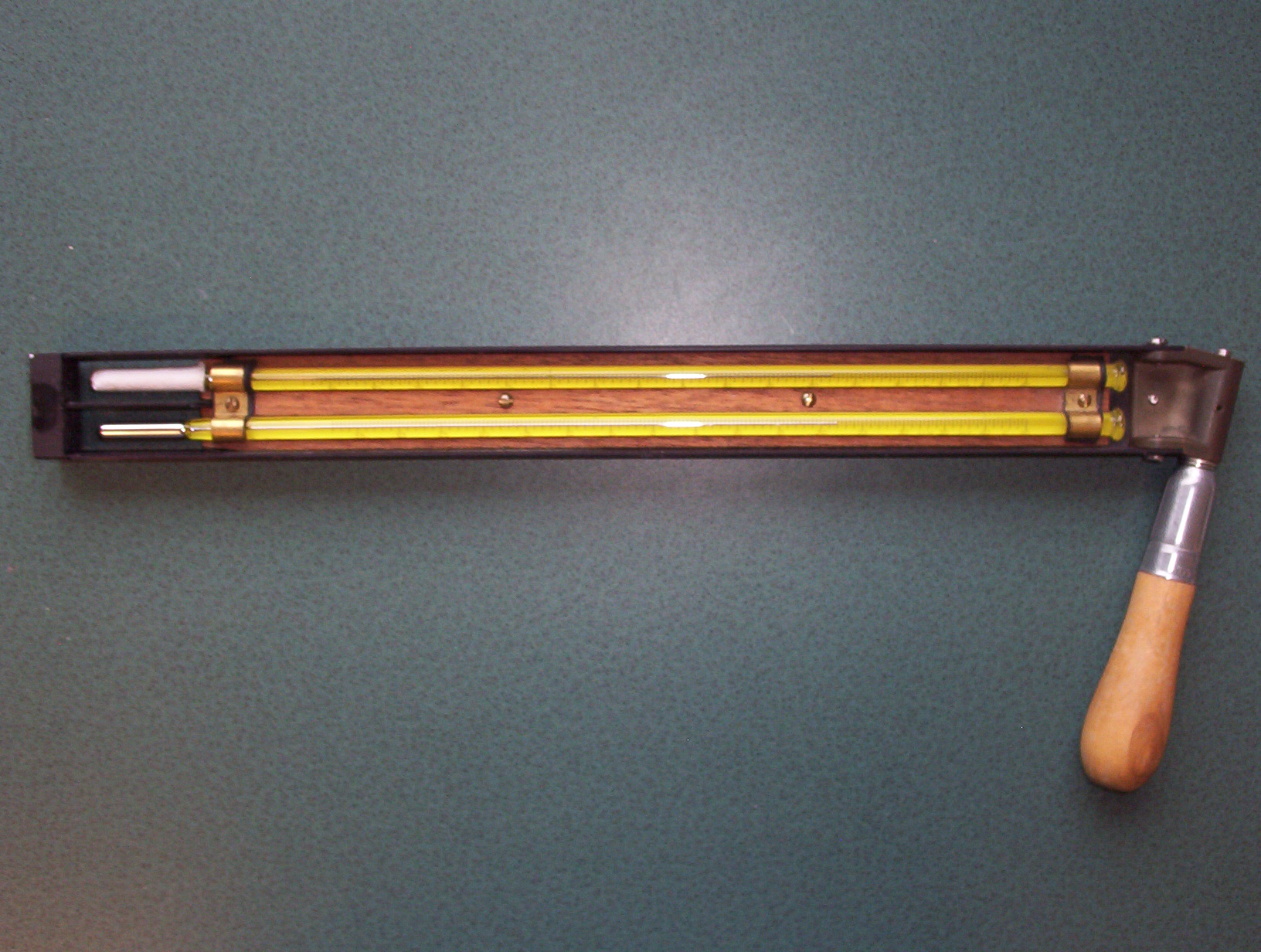
From the sling psychrometer, we can obtain two readings: the dry-bulb temperature (T) and wet-bulb temperature (Tw). The difference between the dry-bulb and wet-bulb temperature is the wet-bulb depression (T-Tw). This is expressed mathematically in Equation 8.1:
[latex]\text{Wet-bulb depression} = T - T_{W} (^{\circ}C).[/latex]
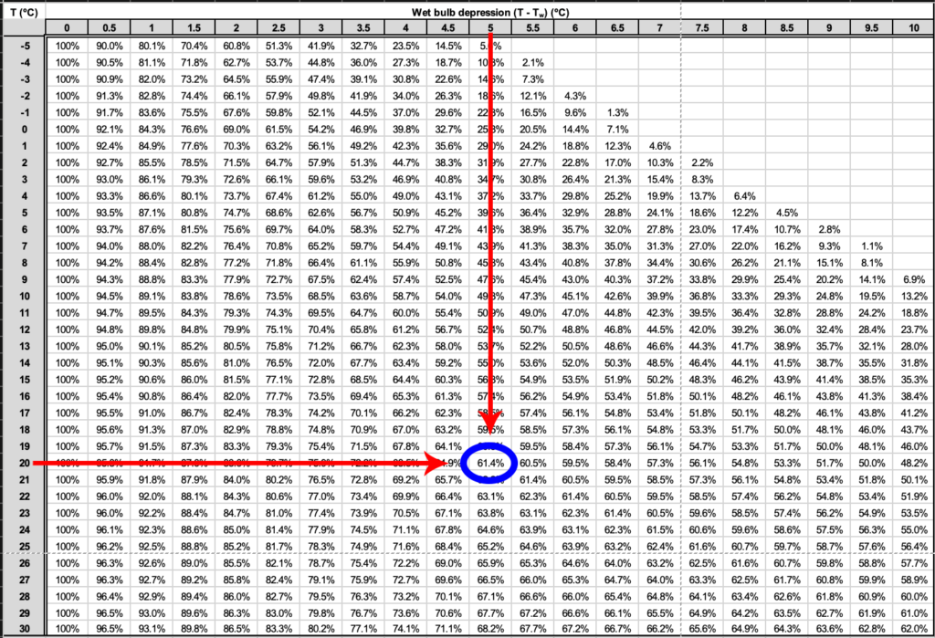
We can then use a psychrometric table to determine the relative humidity (RH) of the air using the four-step procedure described here and illustrated in Figure 8.2:
Step 1: Calculate the wet-bulb depression. If T = 20°C and Tw = 15°C, then using Equation 8.1,
[latex]T - T_{W} = 5^{\circ}C.[/latex]
Step 2: Using the psychrometric table (Table 8.6), look down the first column until you locate the dry-bulb temperature (T = 20°C ).
Step 3: Still using the table, look across until you locate the wet-bulb depression calculated in Step 1.
Step 4: Trace lines across from T and down from T−Tw. The RH is found where these lines intersect. In this example, RH = 61.4%.
We can also use Table 8.7 to help us determine other variables. For example, if T = 20°C, then Table 8.7 shows us that the saturation vapour pressure (es) is 2338 Pa.
Relative humidity can be calculated from vapour pressure using Equation 8.2:
[latex]RH (\%) = \dfrac{e \hspace{2pt} (Pa)}{e_s \hspace{2pt} (Pa)} \times 100\%[/latex],
We can calculate the actual vapour pressure (e) by rearranging Equation 8.2:
[latex]e \hspace{2pt} (Pa) = 2338 \hspace{2pt} Pa \times \dfrac{61.4}{100} = 1436 \hspace{2pt} Pa.[/latex]
Now that we have e = 1436 Pa, we can obtain the dew-point temperature (Td) from Table 8.7. By inspection of the table, we can see that e = 1436 Pa is between the values 1402 Pa and 1498 Pa, and hence Td is between 12°C and 13°C (specifically, 12.35°C by linear interpolation).
Atmospheric Stability
Concepts
Atmospheric stability helps determine whether clouds (and precipitation) form or not. The atmosphere could be
- stable, and so the air parcel remains stationary,
- unstable, and the air parcel either rises or sinks, or
- conditionally unstable.
A key to understanding atmospheric stability is the adiabatic process. An adiabatic process is one in which air is heated or cooled due to expansion or contraction but without addition or subtraction of heat. Air will heat or cool at the dry adiabatic lapse rate (DALR = 10°C/1000m) when the relative humidity is less than 100%. When the relative humidity is 100% (i.e. saturated air), air heats or cools at the moist/saturated adiabatic lapse rate (MALR = 6°C/1000m on average but varies between 5-9°C/1000m).
In Lab 03, you were introduced to the ideas of a sounding and the Environmental Lapse Rate (ELR). The temperature data of the lower atmosphere is typically measured by a weather balloon. Twice a day, meteorologists release a weather balloon to measure temperatures at different elevations. The data are transmitted back to the ground where meteorologists can determine the stability.
To recap, the ELR is calculated using Equation 8.3:
[latex]ELR \hspace{2pt} (^{\circ} C/1000 \hspace{2pt} m) = -1000 \left( \dfrac{\Delta T (^{\circ} C)}{\Delta z (m)} \right) = -1000 \left( \dfrac{T_{2} - T_{1}}{z_{2} - z_{1}} \right)[/latex]
where
- Δ = delta symbol, represents the change in the variable it precedes (for example, the change in temperature)
- T = air temperature (°C)
- z = altitude (m)
- T1 , z1 = the measurement taken at the lower point in the atmosphere
Note that the ELR is also commonly presented with the units °C/1000m and so the equation differs slightly compared to the way it was presented in Lab 03.
To determine atmospheric stability, meteorologists compare the adiabatic lapse rate of an air parcel (either DALR and/or MALR) with the environmental lapse rate (ELR). There are three possible conditions:
- If ELR > DALR > MALR, there is absolute instability (unstable).
- If DALR > ELR > MALR, there is conditional instability (conditionally unstable).
- If DALR > MALR > ELR, there is absolute stability (stable).
Finally, as dry air parcels rise, they cool at the DALR until the dew-point temperature is reached. The elevation at which the dew-point is reached is the Lifting Condensation Level (LCL). The LCL can be calculated using Equation 8.4:
[latex]LCL \hspace{2pt} (m) = \dfrac{T (^{\circ}C)-T_{d}(^{\circ}C)}{DALR \hspace{2pt} (^{\circ} C/1000 \hspace{2pt} m)}[/latex]
where T is the temperature of the air parcel and Td is the dew-point temperature of the air parcel at the surface, both in °C.
The final calculation that we may wish to do is to calculate temperature at a specific altitude with a known lapse rate, and known change in altitude. The temperature at a specific altitude (Tz) can be calculated using Equation 8.5:
[latex]T_{z} \hspace{2pt} (^{\circ} C) = T_{Initial}(^{\circ} C) \pm \Big[ {|\Delta z (m)|} \times \text{Lapse Rate} \hspace{2pt} (^{\circ} C/1000 \hspace{2pt} m) \Big][/latex]
The lapse rate may be the DALR or MALR as appropriate. Add (+) to TInitial when Tz is at a lower altitude than TInitial, and subtract from TInitial when Tz is at a higher altitude.
Application
Let us put all these concepts together with an example. Assume that the data transmitted by a weather balloon are presented in Table 8.1. We can then use the following seven-step process to visualize what will happen to an air parcel as it rises through the atmosphere.
| Altitude (m) | Temperature (°C) |
|---|---|
| 0 | 25.0 |
| 200 | 22.8 |
| 450 | 20.0 |
| 600 | 18.4 |
| 800 | 16.6 |
| 1050 | 14.4 |
| 1200 | 13.1 |
| 1400 | 12.1 |
| 1550 | 11.3 |
| 1800 | 9.9 |
| 2000 | 8.8 |
Step 1: Transfer the data onto the Atmospheric Stability Analysis Form.
Step 2: For each layer of the atmosphere, determine the change in altitude (∆z) and change in temperature (∆T). For example, layer 1 is between 0 m (z1) and 200 m (z2), and so:
[latex]\Delta z = 200 m - 0 m = 200 m[/latex]
[latex]\Delta T = 22.8^{\circ} C – 25.0^{\circ} C = -2.2^{\circ} C[/latex].
Values for all layers are presented in Table 8.2.
Step 3: Determine the ELR of all layers of the atmosphere using Equation 8.3. For example, for layer 1,
[latex]ELR \hspace{2pt} (^{\circ} C/1000 \hspace{2pt} m) = -1000 \left( \dfrac{\Delta T(^{\circ} C)}{\Delta z(m)} \right) = -1000 \left( \dfrac{-2.2^{\circ}C}{200m} \right) = 11.0 ^{\circ} C/1000 \hspace{2pt} m.[/latex]
Values for all layers are presented in Table 8.3.
Step 4: Determine the stability of all layers of the atmosphere by comparing the values of the ELR to the DALR and MALR. For example, for layer 1, the ELR is 11.0°C, which is greater than both the DALR and the MALR. The layer is therefore unstable. Values for all layers are presented in Table 8.4.
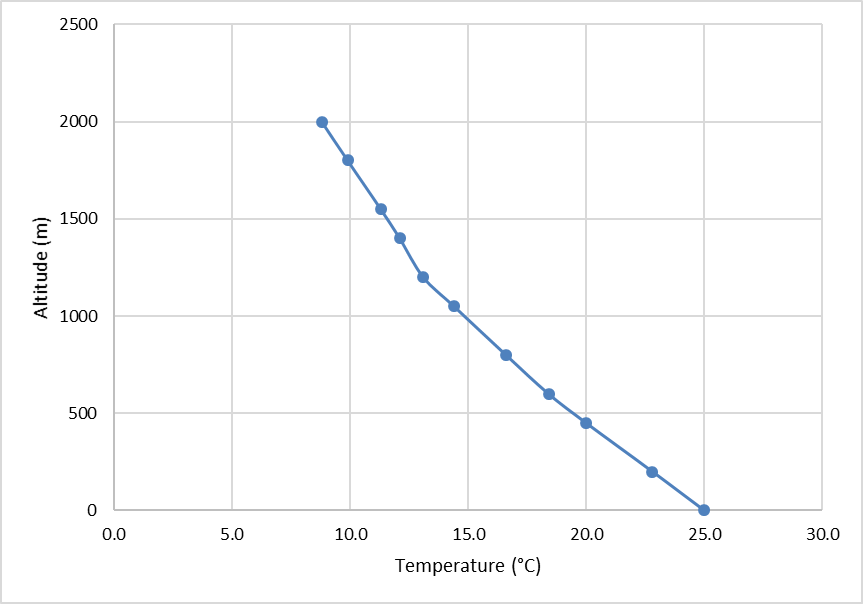
Step 5: Once the Atmospheric Stability Analysis Form is completed, we can plot an atmospheric sounding similar to the one you did in Lab 03. This will help us analyze what could happen to an air parcel. First, plot the temperature data as a line with markers (Figure 8.3).
Step 6: Calculate the change in temperature of an imaginary air parcel as it rises from the ground to 2000 m elevation.
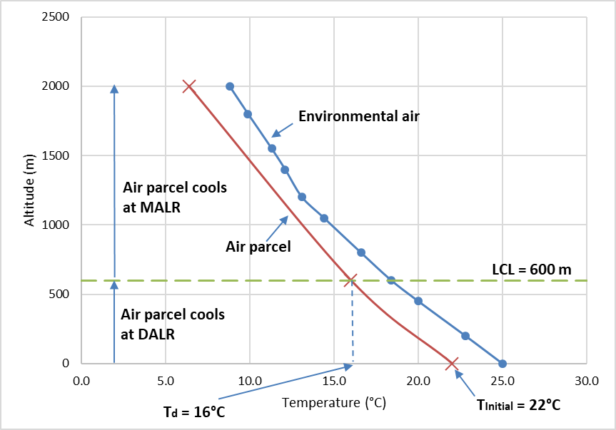
- First up, we need to decide if the air parcel is saturated or not (i.e., RH > 100% or RH < 100%). The air parcel has a temperature (T) of 22°C and dew-point temperature (Td) of 16°C at the surface. Because T is greater than Td, we know that the air parcel is not saturated with water vapour (i.e. RH < 100%). It will therefore cool at the DALR as it rises until the dew-point temperature is reached.
- So, we need to calculate the LCL using Equation 8.4 for this air parcel to determine the altitude at which the dew-point temperature is reached. In this example,
[latex]LCL \hspace{2pt} (m) = \dfrac{T (^{\circ}C)-T_{d}(^{\circ}C)}{DALR \hspace{2pt} (^{\circ} C/1000 \hspace{2pt} m)}[/latex]
[latex]LCL \hspace{2pt} (m) = \dfrac{22^{\circ} C - 16^{\circ} C}{10^{\circ} C/1000 \hspace{2pt} m}[/latex]
[latex]LCL \hspace{2pt} (m) = \dfrac{6^{\circ} C}{10^{\circ} C/1000 \hspace{2pt} m}[/latex]
[latex]LCL \hspace{2pt} (m) = 6^{\circ} C \left( \dfrac{1000 \hspace{2pt} m}{10^{\circ} C} \right)[/latex]
[latex]LCL \hspace{2pt} (m) = 600 \hspace{2pt} m.[/latex]
c. Once the air parcel reaches its LCL, the rate of cooling slows to the MALR, and so we now need to calculate the temperature of the air parcel at 2000 m (Tz) using the MALR and Equation 8.5. In this example, TInitial = Td = 16°C, and z1 = LCL = 600 m:
[latex]T_{z} \hspace{2pt} (^{\circ} C) = T_{Initial}(^{\circ} C) \pm \Big[ {|\Delta z (m)|} \times \text{Lapse Rate} \hspace{2pt} (^{\circ} C/1000 \hspace{2pt} m) \Big][/latex]
[latex]T_{z=2000m} \hspace{2pt} (^{\circ} C) = 16^{\circ} C - \left[|600m - 2000m| \times \dfrac{6^{\circ}C}{1000m}\right][/latex]
[latex]T_{z=2000m} \hspace{2pt} (^{\circ} C) = 16^{\circ} C - \left[1400m \times \dfrac{6^{\circ}C}{1000m}\right][/latex]
[latex]T_{z=2000m} \hspace{2pt} (^{\circ} C) = 16^{\circ} C - 8.4^{\circ} C[/latex]
[latex]T_{z=2000m} \hspace{2pt} (^{\circ} C) = 7.6^{\circ}C[/latex]
Step 7: Plot the change in temperature of this air parcel and the LCL on the atmospheric sounding. Select a different colour and/or different line marker or style for each line. Label each component of the plot. The result is shown on Figure 8.4.
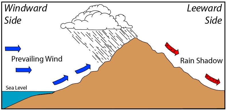
Orographic Lifting
An orographic lifting process is where an air parcel is forced to go over a geographic barrier such as a mountain. When the air parcel ascends on the sea side of the mountain (blue arrows), air cools adiabatically until it reaches the Lifting Condensation Level (LCL). Consequently, air becomes saturated and water vapour condenses to form clouds. As air descends on the leeward side of the mountain (red arrows with hatching), it warms adiabatically at the DALR. Figure 8.5 illustrates this concept.
We can use the relationships presented above to calculate the the change in temperature of an air parcel as it moves through the orographic process. For example, assume an air parcel at sea-level has temperature of 20°C and dew-point temperature of 15°C. This air parcel is forced to rise over a mountain that is 2000 m high and descend back to sea-level on the other side of the mountain (leeward side).
Step 1: Determine the LCL using Equation 8.4:
[latex]LCL \hspace{2pt} (m) = \dfrac{T (^{\circ}C)-T_{d}(^{\circ}C)}{DALR \hspace{2pt} (^{\circ} C/1000 \hspace{2pt} m)} = \dfrac{20^{\circ} C - 15^{\circ} C}{10^{\circ} C/1000 \hspace{2pt} m} = 500 \hspace{2pt} m[/latex]
Step 2: Determine the temperature of the air parcel when it reaches the summit using Equation 8.5:
[latex]T_{z} \hspace{2pt} (^{\circ} C) = T_{Initial}(^{\circ} C) - \Big[{|\Delta z (m)|} \times MALR \hspace{2pt} (^{\circ} C/1000 \hspace{2pt} m) \Big][/latex]
[latex]T_{z=2000m} \hspace{2pt} (^{\circ} C) = 15^{\circ} C - \left[|500m - 2000m| \times \dfrac{6^{\circ}C}{1000m} \right] = 6^{\circ}C[/latex]
Step 3: Determine the temperature of the air parcel when it sinks back to sea-level on the other side of the mountain (leeward side) using Equation 8.5:
[latex]T_{z} \hspace{2pt} (^{\circ} C) = T_{Initial} (^{\circ} C) + \Big[{|\Delta z (m)|} \times DALR \hspace{2pt} (^{\circ} C/1000 \hspace{2pt} m) \Big][/latex]
[latex]T_{z=0m} = 6^{\circ} C + \left[|2000m - 0m| \times \dfrac{10^{\circ}C}{1000m}\right] = 26^{\circ}C[/latex]
Lab Exercises
In this lab, you will be doing a number of different calculations to help you understand the concepts of atmospheric moisture and stability. You will:
- Convert between moisture variables and related temperatures.
- Relate atmospheric moisture to your own comfort level.
- Analyze atmospheric stability and visually present the information you calculate.
A calculator is required, and you will also be plotting a graph—your instructor will decide if you will use a graph paper or a spreadsheet. Please make sure to show all your calculations (to maximize partial credits) and not just the answers. It is estimated that this lab will take 4-5 hours to complete.
EX1: Moisture Variables
- Complete Table 8.5. It is also available for download in Worksheets. Give answers for RH and Td to one decimal place, and e to the nearest integer.
Use Table 8.6 and Table 8.7 in the Supporting Material section. Show your calculations on a separate page.
EX2: Atmospheric Moisture
- On a cold snowy day, the outside air temperature is 0°C and the relative humidity is 100%. The air is taken into the house and heated to 21°C. What is the relative humidity inside the house?
- Dew is often formed on grass early in the morning but not at other times of the day. Explain why this is.
- Go to Historical Data Report for Vancouver International Airport. Check that the date matches today’s date. Have a look at the relative humidity. Next, click the Previous Day button located to the left of the date bar, and track the relative humidity over the preceding 3-4 days. Think back to how you felt over those days. Do you feel more comfortable when the RH is high, or low? Explain the major factors that affect RH.
- Search online to acquire the company names and model numbers of at least two different instruments (other than the sling psychrometer) for sensing humidity.
EX3: Atmospheric Stability
- A meteorological balloon is sent aloft and temperature data are obtained. Your instructor will provide you with this data, or instructions on how to obtain it.
- Open the Atmospheric Stability Analysis Form in Worksheets and enter the temperature and altitude data.
- Plot the vertical temperature profile (sounding) using Excel. If required, step-by-step instructions on how to do this are provided in Lab 03 EX1 Step 4.
- Label this line Environmental Air.
- Label the axes of your graph. Include units.
- Complete the Atmospheric Stability Analysis Form. Give your answers for ELR to one decimal place. Assume a DALR of 10°C / km and an MALR of 6°C / km.
- An air parcel of 24°C and dew-point temperature of 16°C is currently hovering at the surface. The air parcel is forced to rise up to an altitude of 2000 m.
- Calculate the lifting condensation level (LCL). Add the LCL to your graph.
- Plot a line showing the hypothetical change in temperature of this rising parcel on your graph.
- Label this line Air Parcel. On the line indicate where the rising parcel of air cools at the DALR and where it cools at the MALR.
Submit the Atmospheric Stability Analysis Form and your graph as directed by your instructor.
EX4: Orographic Process
Air blowing off the Pacific Ocean has a temperature of 15°C and a dew-point temperature of 10°C at Vancouver (sea level). This air is forced to rise over the Coast Range on its way to Calgary.
- What is the LCL of the air blowing off the Pacific Ocean at Vancouver?
- What is the temperature of the air parcel at the top of the Coast Range (z = 2200 m)?
- What is the temperature of the air parcel in Calgary (z = 1200m)?
Show your calculations.
Reflection Questions
- If we changed the temperature of the air parcel in Vancouver to 30°C and dew-point temperature to 7°C in EX4, what would the temperature of the air parcel be when it reaches Calgary? Explain what will happen in 2-3 sentences.
- Condensation, as occurs at the LCL, is one example of phase change. Take a picture of something around you that illustrates one of the processes of phase change. Take the photo at home or somewhere outside. Include one or two sentences to describe what that example is. Do not use a scenario that has already been discussed in class.
- Draw a line on the picture in Figure 8.5 indicating where the Lifting Condensation Level (LCL) is. Explain your reasoning in 2-3 sentences.
Worksheets
EX1 Worksheet – Table 8.5
Atmospheric Stability Analysis Form
- Lab 08 Atmospheric Stability Analysis Form [Word]
- Lab 08 Atmospheric Stability Analysis Form [Excel]
- Lab 08 Atmospheric Stability Analysis Form [ODT]
- Lab 08 Atmospheric Stability Analysis Form [PDF]
Supporting Material
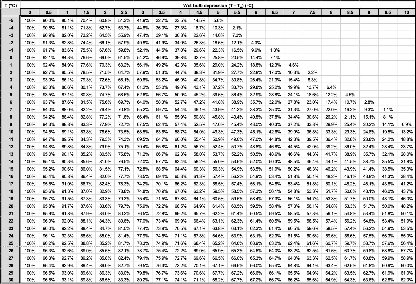
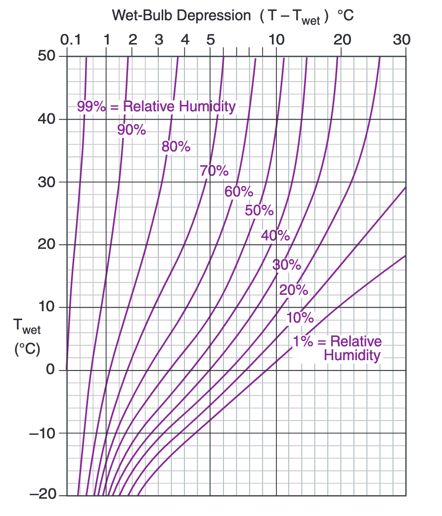
Figure 8.6. Psychrometric Graph
References
Geography Department, Langara College.(2017). Geography 1180 Lab Manual.
Stull, R. (2017). Practical meteorology: An algebra-based survey of atmospheric science, version 1.02b. University of British Columbia.
