Chapter II: Mineral Processing
4. Size Distribution
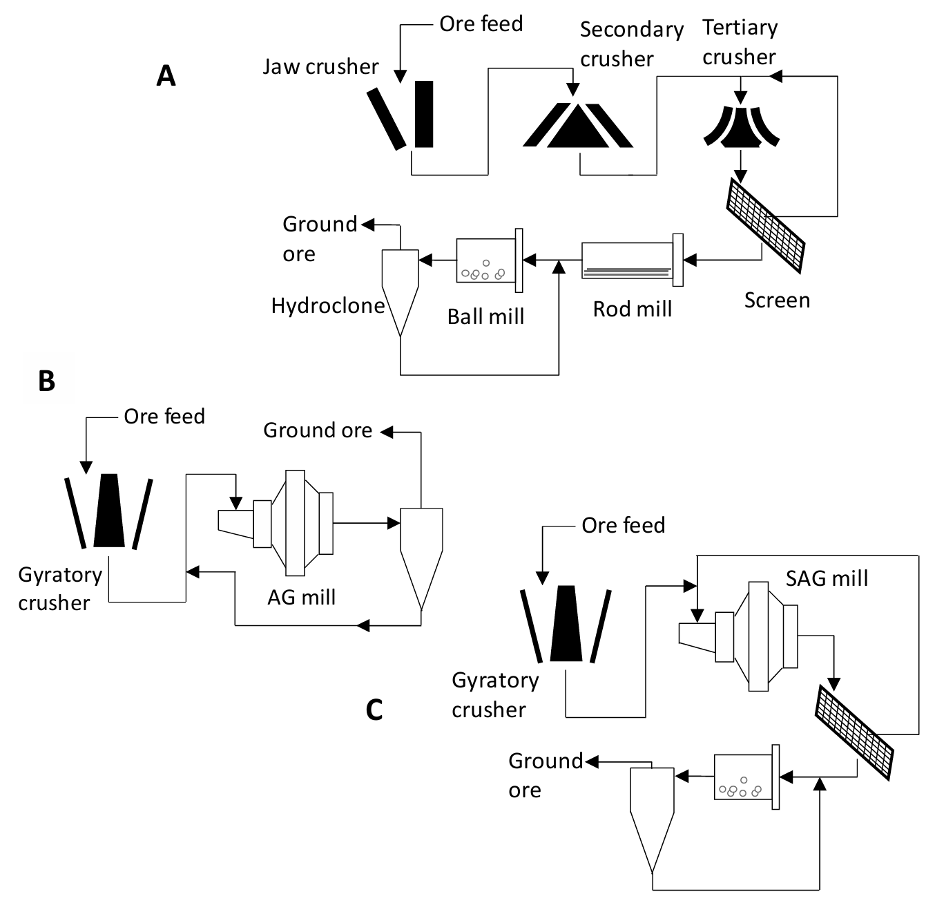
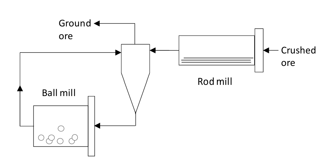
Size reduction processes produce a range of particles sizes as indicated qualitatively in Figure 4.1 (below). It is important to know the size distribution of a crushed or ground ore that is being fed to the next steps in an extractive metallurgy process. Particle size has significant influences on concentration processes and leaching processes. Too small or too big and there can be significant losses in recovery of minerals or metals. Size distribution strongly affects rates of leaching processes. In heap leaching too much fine material can prevent solution flow, plugging heaps.
Size analysis can be performed using automated equipment. For example, some size analysis instruments work on the principle of scattering of light. Different sizes scatter light to different extents. A laser light source is used. Careful calibration with known materials is required. A continuous size distribution plot (fraction of particles versus size) is obtained and the analysis can be done fairly quickly.
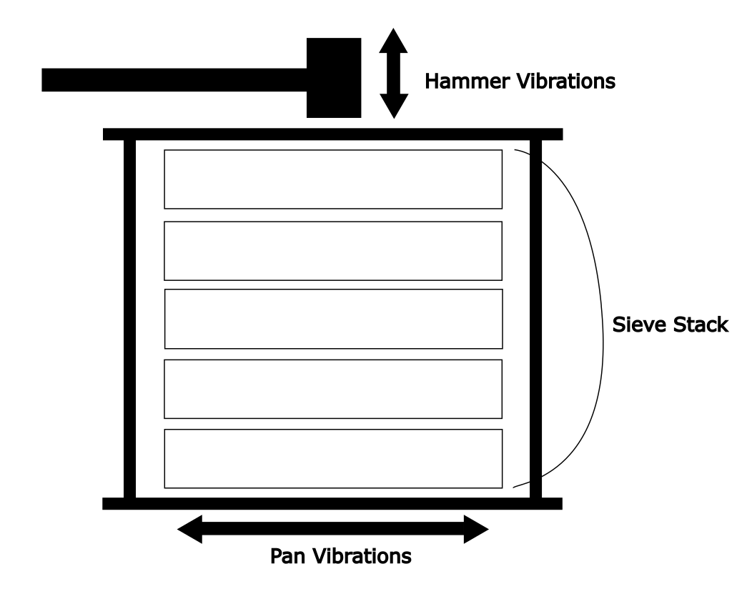
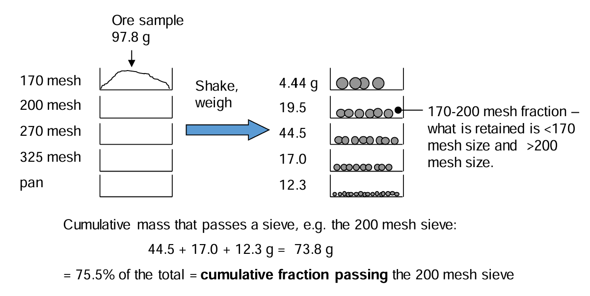
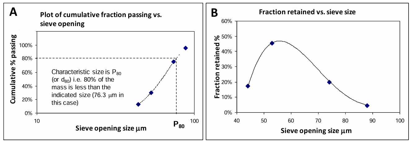
A simple and commonly practiced size analysis technique is laboratory screening. A known mass of sample is introduced onto the top of a stack of sieves of varying opening sizes. The coarsest sieve is at the top, the finest is the second to last near the bottom. A pan is placed at the bottom of the stack to capture any material too fine to be retained by the finest sieve. The sieve stack is vibrated to facilitate passage of particles through the sieves (see Figure 4.3). Dry or wet sieving may be employed depending on the material and its size range. Wet sieving uses water to help carry the smallest particles down through the sieves with larger openings. At the end, each sieve is weighed (after drying if wet sieving was used) to determine the mass of ore retained by the sieve. Each sieve holds particles too big to pass through it and small enough to have passed through the sieve above. From this data the size distribution can be plotted. Each point represents a range of sizes. For instance if 7.75 g was retained by a 150 mesh sieve (105 μm) and the sieve above it was a 100 mesh sieve (149 μm), and the total mass of ore screened was 98.1 g then 7.75/98.1 = 7.90% of it was >105 μm and less than 149 μm (- 149 μm to +105 μm). Obviously the greater the number of sieves used, the better the resolution of the distribution curve. Regardless though, the analysis is discrete rather than continuous. Figure 4.4 shows an example of a sieve analysis. Table 4.1 illustrates the kind of data that is obtained. Figure 4.5 shows how the data can be plotted to obtain size distributions. Note that P80 is upper size below which 80% of the material resides. It's a common characteristic of a size distribution.
Size analysis is prone to some errors that require care to correct or avoid. Sieve opening size for the same mesh may vary somewhat between manufacturers. Calibration using known size glass beads can lower this error. Screen opening sizes can be non-uniform. Misuse and rough handling or cleaning is a potential cause. If a ground material passes through in a matter of minutes and then there is no further material passing, the sieve is quite uniform. Too much sample is a common source of errors. Apparently 50-100 g for 8 inch diameter sieves is suitable. There are methods to test for errors caused by too much sample. It is challenging to obtain a representative sample from a large mass of a ground material. Wet sieving may be necessary when fine material can clump and then not pass through fine sieves. It may also be preferable for sieving fragile minerals. Standard methods for sieve analysis are available.
| Table 4.1 - Data and calculations for a sieve analysis | ||||||
|---|---|---|---|---|---|---|
| Sieve (mesh) | Opening (micrometer) | Mass retained (g) | Fraction retained % | Log10 | Cumulative mass passing sieve (g) | Cumulative fraction passing % |
| 170 | 88 | 4.44 | 4.5 | 1.94 | 93.36 | 95.5 |
| 200 | 74 | 19.53 | 20.0 | 1.87 | 73.83 | 75.5 |
| 270 | 53 | 44.5 | 45.5 | 1.72 | 29.32 | 30.0 |
| 325 | 44 | 17.00 | 17.4 | 1.64 | 12.32 | 12.6 |
| 12.32 | 12.6 | |||||
| Total | 97.8 | |||||
Media Attributions
- Ch2_F22_Size_Reduction_Circuits © Bé Wassink and Amir M. Dehkoda is licensed under a CC BY-NC (Attribution NonCommercial) license
- Ch2_F23_Size_Classifier © Bé Wassink and Amir M. Dehkoda is licensed under a CC BY-NC (Attribution NonCommercial) license
- Ch2_F24_Sieve_Shaker © Bé Wassink and Amir M. Dehkoda adapted by Jeno Hwang is licensed under a CC BY-NC (Attribution NonCommercial) license
- Ch2_F25_Sieve_Analysis © Bé Wassink and Amir M. Dehkoda is licensed under a CC BY-NC (Attribution NonCommercial) license
- Ch2_F26_Size_Distribution_Graphs © Bé Wassink and Amir M. Dehkoda is licensed under a CC BY-NC (Attribution NonCommercial) license
