Chapter III: Introduction to Eh pH Diagrams
4. Constructing Eh-pH Diagrams
4.1 The Water Eh-pH Diagram
Half Reactions and Data
In order to be able to make use of Eh-ph diagrams for aqueous solutions, we need to know what the stability of water is with potential and pH. Water can be reduced (to form H2) and it can be oxidized (to form O2). In terms of reductions alone, which is what we will be plotting, O2 can be reduced to water. First we have to write suitable half reactions. Consider water reduction to H2. Here we must simply follow the rules for balancing reactions:
[latex]\begin{align*} \ce{H2O}&=\ce{H2} \\ \ce{H2O}&=\ce{H2}+\ce{H2O} \\ \ce{H2O}&+\ce{2H+}=\ce{H2}+\ce{H2O} \\ \ce{\cancel{H2O}}&+\ce{2H+}+\ce{2e-}=\ce{H2}+\ce{\cancel{H2O}} \\ \ce{2H+_{aq}}&+\ce{2e-}=\ce{H2_g}\tag{67} \end{align*}[/latex]
This means that water reduction is equivalent to H+ reduction. The reduction of O2 to form water is,
\[\ce{O2_g + 4H^{+}_{aq} + 4e^- = 2H2O_l} \tag{68}\]
We also need ΔG°f data: ΔG°f(H2O) = -237.15 kJ/mol. For all the other species, ΔG°f = 0 by definition. Then we obtain ΔG° for each half reaction:
\[\text{For }\ce{2H+_{aq} + 2e^- = H2_g}\quad \Delta G^{\circ} = 0 - 0 = 0\ \text{kJ/mol} \tag{69}\]
\[\text{For }\ce{O2_g + 4H+_{aq} + 4e^- = 2H2O_l}\quad \Delta G^{\circ} = 2 \times (-237.15) = -474.30\ \text{kJ/mol} \tag{70}\]
Now the gas pressures must be specified. This depends entirely on what conditions one is interested in; for an autoclave we might be dealing with 100 atm, and for an open tank, perhaps 1 atm. First we will set gas pressures to be 1 atm. The only ion involved is H+, and its activity is incorporated into the pH term.
Calculating the Eh Equations
Starting with the H+/H2 half reaction and using the Eh equation,
\[\;E_h = -\frac{\Delta G^{\circ}}{nF} - \frac{2.303RT}{nF}\log Q_H - \frac{2.303RT\,m}{nF}\,pH \tag{71}\]
m = 2 and n = 2; T = 25°C = 298.15 K:
\[\;E_h = 0 - \frac{2.303RT}{nF}\log(P_{H_2})
- \frac{2.303 \times 8.314 \times 298.15 \times 2}{2 \times 96485}\,pH
\tag{72}\]
\[\;E_h = -0.02958\log(P_{H_2}) - 0.05917\,pH = -0.05917\,pH \text{ when } P_{H_2}=1\ \text{atm} \tag{73}\]
Thus Eh = 0 at pH = 0, as expected, based on E°H+/H2 = 0. For the O2/H2O couple,
\[\;E_h
= -\frac{474{,}300\ \text{J/mol}}{2\ \text{mol e}^-/\text{mol} \times 96485\ \text{C/mol e}^-}
- \frac{2.303RT}{nF}\log\!\left(\frac{1}{P_{O_2}}\right)
- \frac{2.303 \times 8.314 \times 298.15 \times 4}{4 \times 96485}\,pH
\tag{74}\]
Note that DG° must be converted to J/mol from kJ/mol.
\[\;E_h = 1.229 - 0.01479\log\!\left(\frac{1}{P_{O_2}}\right) - 0.05917\,pH
= 1.229 - 0.05917\,pH \tag{75}\]
when PO2 = 1 atm.
These two equations can be plotted on a graph, as in Figure 4.1 (below). The resulting diagram is the Eh-pH diagram for water at 25°C and 1 atm pressure. Below the H+/H2 line, water will be converted into H2 (e.g. if a reducing agent with Eh < EhH+/H2 is added it will yield electrons to the oxidant, H+, and form H2).
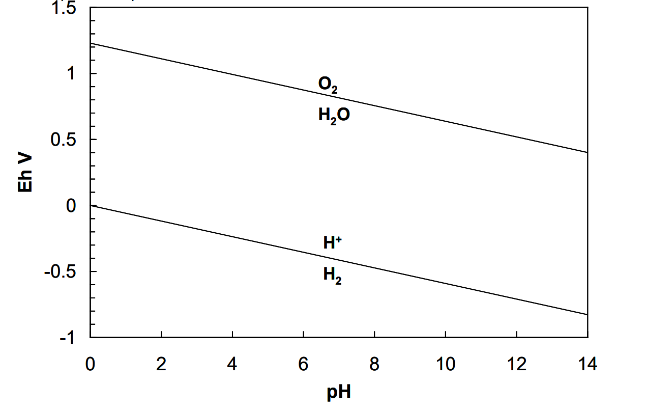
And, above the O2/H2O line, water will be converted into O2. It is important to bear in mind that the lines are plots of half reaction potentials, relative to standard H+/H2 versus pH. It tells us, for instance, that if we add a strong oxidant, like KMnO4 (E°MnO4-/Mn+2 = 1.51 V in acid solution) to water at pH 0, it should oxidize it to form O2 and Mn+2. This does occur, although very slowly. It tells us that water becomes increasingly prone to oxidation as pH rises. And, it tells us that water becomes progressively more stable toward reduction as pH rises. Thus, anywhere between the lines water is thermodynamically stable. The diagram shows us the Eh-pH domain over which water is stable, i.e. is the dominant species.
Understanding the Diagram
There are some important subtleties to take note of. For one, pure liquid water has an activity of 1 by definition (as do all pure solids and liquids). Between and on the lines water has unit activity. This means that above the O2/H2O line or below the H+/H2 line water will not exist at all, at least thermodynamically speaking, since it can have activity of either 1 (pure water) or 0 (no water left). Practically, this would require that the oxidant, for instance, react rapidly with water. But, thermodynamically speaking, water is completely unstable outside its region of stability. These considerations apply to any pure solid or liquid.
Second, H2 and O2 can have varying pressures, so they can in principle exist in contact with water, i.e. within the stability region for water. For instance, if we maintain a potential of 0.2 V at pH 0 in water (for example by introducing a suitable redox couple, such as Ru+3/Ru+2; E° = 0.24 V and with a suitable reaction quotient aRu+2/aRu+3) we can calculate what the H2 pressure can be. Now we must allow for a PH2 different from 1 atm:
\[\;E_h
= -\frac{2.303 \times 8.314 \times 298.15}{2 \times 96485}\log P_{H_2}
- \frac{2.303 \times 8.314 \times 298.15 \times 2}{2 \times 96485}\,pH
\tag{76}\]
\[\;E_h = 0.20\ \text{V} = -0.02958\log P_{H_2} - 0.05917\,pH \tag{77}\]
Solving for PH2 at pH 0 gives PH2 = 4.17 x 10⁻⁴ atm. This is considerably less than 1 atm, which is what the pressure was on the line (which we used to calculate the line). So species that can have variable activity (like gases and solutes) do exist within the region of dominance for another species, but at lower activities than the dominant species. Therefore, a region on an Eh-pH diagram shows the Eh-pH domain over which that one species is the predominant one.
The lines shift if we change the pressures of the gases. If we increase PH2, for instance, the effect in equation (76) will be to decrease the Eh. Likewise, increasing PO2 in equation (74) will increase the Eh. The net effect is to make water more stable, increasing the size of the water region. However, the effect is small; at 10 atm the H+/H2 line shifts down by 0.03 V and the O2/H2O line shifts up by 0.015 V.
Why Other H-O Compounds Were Not Included
Finally, there are O, H chemical species that we might have considered, such as O3 (ozone gas) and H2O2 (hydrogen peroxide). Consider the sequence of half reactions,
\[\ce{O2_{g} + 2H+^{ }_{aq} + 2e- = H2O2_{aq}}\tag{78}\]
\[\ce{H2O2_{aq} + 2H+^{ }_{aq} + 2e- = 2H2O_{l}}\tag{79}\]
Thus O2 could be reduced first to H2O2, then H2O2 to water. This suggests the possibility of two different lines (couples) on the Eh-pH diagram: O2/H2O2 and H2O2/H2O. For this to actually occur, Eh for the O2/H2O2 couple would have to be greater than that for the H2O2/H2O couple. We'll see why. The ΔG°f value for H2O2 aq is -133.68 kJ/mol at 25°C. The Eh equations can be calculated for the couples using equation (71) and plotted on an Eh-pH diagram. This is shown in Figure 4.4. Note that thermodynamically speaking H2O2 at unit activity is able to oxidize water, so it should not survive in water at any pH, and we could thus leave it off the diagram. (However, H2O2 has substantial kinetic stability in water, i.e. it reacts with water slowly, so we can make H2O2 solutions.) But, note that if we reduce H2O2 using a suitable reductant we will form water, and at a potential well above Eh for the O2/H2O2 couple. This means that we can't reduce O2 to H2O2 first. Second, if we do try to reduce O2 to H2O2, this will occur at a potential well below the H2O2/H2O couple.
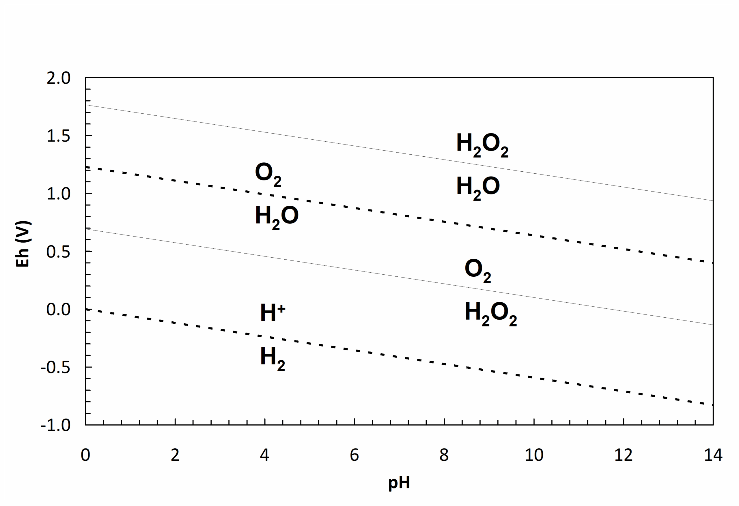
This means that the potential to form H2O is higher and the result will be that we form water rather than H2O2. In short, the couples involving H2O2 are inconsistent with the thermodynamics, and we have no good thermodynamic basis for including them. Finally, note too that the region between the H2O2/H2O and O2/H2O lines suggests that both O2 and H2O are dominant species here. Since this cannot be, it is another clue that the arrangement is untenable. (For a given pair of elements, only one species can be dominant in any given region).
Now that we have the water Eh-pH diagram we can start to build other diagrams for aqueous solutions. The water diagram tells us what is thermodynamically allowable (or not) in aqueous solution.
4.2 The Zinc-Water Eh-pH Diagram
Chemical Species and Data
When we refer to the Zn-H2O diagram, or system, we mean to consider all possible species that contain Zn, O and H. A list of the known species and their corresponding ΔG°f data is provided in Table 4.1 (below). It should be apparent then that such diagrams are only as good as our chemical knowledge of any given system. For this diagram, to start with, we will use unit activities for solutes, 1 atm pressure for gasses and a temperature of 25°C.
| Table 4.1 - Thermodynamic data for Zn–H2O chemical species at 25°C | |
|---|---|
| Species | ΔG°f kJ/mol |
| Zn s | 0 (by definition) |
| Zn+2aq | -147.2 |
| ZnO s | -318.3 |
| HZnO 2-aq | -463.9 |
| ZnO22-aq | -389.1 |
| H2O l | -237.15 |
| H+aq | 0 (by definition) |
Assigning Oxidation States
At this stage we need to determine the oxidation states of the species. The reason is that we would expect more highly oxidized species to appear at higher reduction potentials, and more reduced species to appear at lower potentials. This will give us a rough sense of what to expect. In addition some species may have the same oxidation state. This will mean that they are related to each other by non-electron transfer reactions (acid-base processes). Oxidation states can be assigned by the traditional rules. This was presented in the Chemistry Review Part I course notes. Another simple way to do it is to write a half reaction for the reduction of the compound/ion to the principal element (Zn here). To illustrate:
\[
\ce{HZnO2^- = Zn} \qquad \tag{80}
\]
\[
\ce{HZnO2^- = Zn + 2H2O} \qquad \tag{81}
\]
\[
\ce{HZnO2^- + 3H^+ = Zn + 2H2O} \qquad \tag{81}
\]
\[
\ce{HZnO2^-_{aq} + 3H^+_{aq} + 2e^- = Zn_{s} + 2H2O_{l}} \qquad \tag{83}
\]
Next, divide the number of electrons (2 here) by the number of metal atoms involved in the reaction (1 Zn here). This gives a value of 2. The oxidation state for Zn in this ion then is +2.* The oxidation state for each of Zn+2 (obviously +2), ZnO, HZnO2- and ZnO22- is +2. The oxidation state for the element is always 0 by definition. This means that we would expect a diagram with Zn at the bottom and the other four Zn(II) species above. But, what will be the order for the four Zn(II) species? That comes next.
Consider another example. What is the oxidation state of S in H2S? Write the half reaction for reduction to S:
[latex]\ce{H2S = S}[/latex]
[latex]\ce{H2S = S + 2H+}[/latex]
[latex]\ce{H2S_{g} = S_{s} + 2H+_{aq} + 2e-}[/latex]
But, the electrons show up on the right side. Therefore, write the reaction as:
[latex]\ce{H2S_{aq} - 2e- = S_{s} + 2H+_{aq}}[/latex]
which is mathematically equivalent, and now has the form of a reduction half reaction. Finally, divide the number of e- (-2; include the sign!) by the number of involved S in the half reaction (1 here). The oxidation state of S in H2S then is -2.
Hydrolysis Reactions
When metal ions in aqueous solution exhibit acid-base behaviour (and almost all do), we call it hydrolysis, meaning splitting by water. This was introduced in the Chemistry Review Part II course notes. Now we need a more thorough treatment. Consider the triprotic acid H3AsO4. It has three acid dissociable protons.
\[
\ce{H3AsO4_{aq} = H2AsO4^-_{aq} + H^+_{aq}}
\qquad
pK_{a1} = 2.24
\qquad \tag{84}
\]
\[
\ce{H2AsO4^-_{aq} = HAsO4^{2-}_{aq} + H^+_{aq}}
\qquad
pK_{a2} = 6.96
\qquad \tag{85}
\]
\[
\ce{HAsO4^{2-}_{aq} = AsO4^{3-}_{aq} + H^+_{aq}}
\qquad
pK_{a3} = 11.50
\qquad \tag{86}
\]
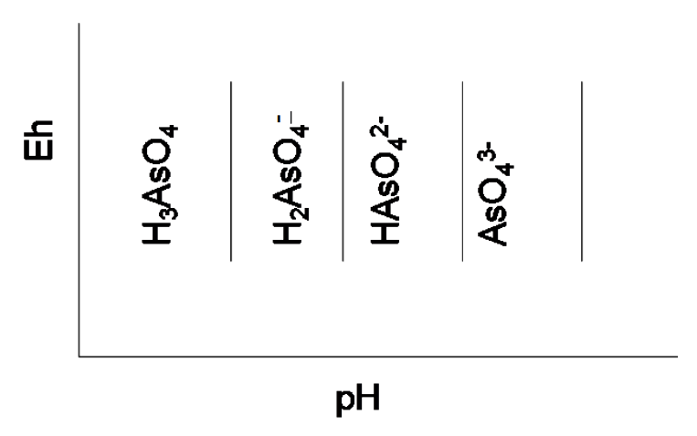
All four species have oxidation state +5. As we might expect, H3AsO4 is the strongest acid, followed by H2AsO4-, followed by HAsO42-. If we were to depict these three reactions on an Eh-pH diagram, there would be three vertical lines; one for each dissociation (no electrons are involved, so the pH at some fixed solute activity would be a constant independent of Eh for each reaction, as we noted previously as a special case in the development the of the Eh equations.)
Now, if we start with AsO43- at high pH and lower the pH (add H+) we would form HAsO42-. This means that AsO43- appears at the highest pH and the species next to it to the left (lower pH) is HAsO42-. At pH 11.50, the buffer point, we would have equal activities (approximately equal concentrations) of both. Since in our Eh-pH diagrams we specify that the solutes have some fixed activity, the pH we would calculate by equation [32] would correspond to pKa3. The same considerations can be applied to lowering the pH and forming H2AsO4- from HAsO42-. Likewise for H2AsO4- and H3AsO4. This means that the strongest acid appears at the lowest pH, followed by the next strongest acid, etc. This is diagrammed in Figure 4.3.
Hydrolysis of metal ions involve reactions such as,
\[\ce{[M(H2O)6]^{2+}_{aq} = [M(H2O)5(OH)]+_{aq} + H+_{aq}} \tag{87}\]
\[\ce{[M(H2O)5(OH)]+_{aq} = M(OH)2_{s} + H+_{aq} + 4H2O_{l}} \tag{88}\]
\[\text{or,}\ \ce{[M(H2O)5(OH)]+_{aq} = MO_{s} + H+_{aq} + 5H2O_{l}} \tag{89}\]
etc. Numerous such dissociations are possible in principle. A more convenient shorthand for the same reactions is:
\[\ce{M^{2+}_{aq} + H2O_{l} = MOH+_{aq} + H+_{aq}} \tag{90}\]
\[\ce{MOH+_{aq} + H2O_{l} = M(OH)2_{s} + H+_{aq}} \tag{91}\]
\[\text{or,}\ \ce{MOH+_{aq} = MO_{s} + H+_{aq}} \tag{92}\]
etc. In almost all cases the hydrated metal ion, Mn+aq is the strongest acid and appears at the lowest pH.
The figure below is a summary of sequential hydrolysis reactions. It can be seen that with increasing extent of hydrolysis (number of acid dissociations) the number of possible metal oxide/hydroxide species increases as well. With each successive dissociation more O or less H resides with the metal. We can call these sequential compounds or ions hydrolysis states, analogous to oxidation states. For any given step only one of the possible species may appear on an Eh-pH diagram. The reason for this is that transformations between species with the same hydrolysis state involve only water, e.g.
\[\ce{M(OH)2_s = MO_s + H2O_l} \tag{93}\]
This was special case 4 in the development of the Eh equations.
| Table 4.2 - Sequential hydrolysis reactions for metal ions and the various possible M-O-H ions and compounds that can form (not all will in any given case). Further subsequent hydrolyses are also possible (5th H+, etc.). | |||
|---|---|---|---|
| 1st H+ | 2nd H+ | 3rd H+ | 4th H+ |
| M2+ + H2O = MOH+ + H+ | MOH+ + H2O = M(OH)2 + H+
MOH+ = MO = H+ ONLY 1 OF THE ABOVE |
M(OH)2 + H2O = M(OH)3 + Ht
MO + H2O = M(O)OH- + H+ MO + 2H2O = M(OH)3 + H+ ONLY 1 OF THE ABOVE |
M(OH)3- + H2O = MH(OH)42- + H+
M(OH)3- = MO(OH)22- + H+ M(OH)3- = MO22- + H2O + H+ M(O)OH- + 2H2O = MO(OH)42- + H+ M(O)OH- + H2O = MO(OH)22- + H+ M(O)OH- = MO22- + H- ONLY 1 OF THE ABOVE
|
| Low pH / Strongest Acid | High pH / Weakest Acid | ||
Calculating Hydrolysis States
The simplest way to assess the order in which the acids go on an Eh-pH diagram, for a given oxidation state, is to calculate the hydrolysis state. (This works mainly for metal oxo- and hydroxy-ions.) This is show below:
\[\mathrm{HS} = \frac{2 \times \text{no. O atoms} - \text{no. H atoms}}{\text{no. metal atoms}} \tag{94}\]
Consider some examples:
\[
\ce{M^{n+}}
\qquad
\mathrm{HS} = 0
\quad
\text{(unhydrolyzed; no acid dissociation has occurred)}\tag{95}
\]
\[
\ce{M(OH)^+}
\qquad
\mathrm{HS} = \frac{2 \times 1 - 1}{1} = 1 \tag{96}
\]
\[
\ce{M(OH)2}
\qquad
\mathrm{HS} = \frac{2 \times 2 - 2}{1} = 2 \tag{97}
\]
\[
\ce{MO}
\qquad
\mathrm{HS} = \frac{1 \times 2 - 0}{1} = 2 \tag{98}
\]
\[
\ce{[Mo7O24]^{6-}}
\qquad
\mathrm{HS} = \frac{24 \times 2 - 0}{7}
= \frac{48}{7}
= 6.857
\qquad \tag{99}
\]
The larger the hydrolysis state, the more H+ that have been released per metal ion, and the weaker an acid the compound/ion is, and the further it appears to the right (higher pH). Thus hydrolyzed metal ions can be arranged from left to right in order of increasing HS. Finally, most metal ions have a small number of hydrolysis states. Some exceptions include oxo/hydroxo ions of V, Mo and W.*
Consider again H3AsO4 and its sequential dissociations. The HS for H3AsO4 is 5. The metal cation alone would be As+5. This is such a high charge that the raw cation will not exist in aqueous solution; it will hydrolyze, in this case to form H3AsO4. For As(V) in aqueous solution the lowest hydrolysis state is 5. The first dissociation forms H2AsO4-, with HS = 6, etc. For the hydrated metal cation M+2, which properly is [M(H2O)n]+2, the hydrolysis state can be calculated to be 0: 2n - 2n.
Tentative Eh-pH Diagram for the Zn-H2O System
The hydrolysis states for Zn(II) species are:
\[
\ce{Zn^{2+}_{aq}}
\qquad
\mathrm{HS} = 0 \tag{100}
\]
\[
\ce{ZnO_{s}}
\qquad
\mathrm{HS} = 2 \tag{101}
\]
\[
\ce{HZnO2^-_{aq}}
\qquad
\mathrm{HS} = 3 \tag{102}
\]
\[
\ce{ZnO2^{2-}_{aq}}
\qquad
\mathrm{HS} = 4
\qquad \tag{103}
\]
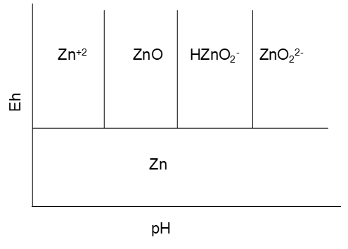
(HZnO2-is probably better presented as Zn(O)OH-.) This then suggests a preliminary Eh-pH diagram as shown in Figure 4.4 (below).
Calculating the pH of the Hydrolysis Reactions
It is often best to start by calculating the hydrolysis pH lines. There is no Zn(OH)+ species listed, so we go directly from Zn+2 to ZnO. The reactions are:
Step 1
\[
\ce{Zn^{2+} = ZnO}\tag{104}
\]
\[
\ce{Zn^{2+} + H2O = ZnO} \tag{105}
\]
\[
\ce{Zn^{2+}_{aq} + H2O_{l} = ZnO_{s} + 2H^+_{aq}}
\qquad \tag{106}
\]
\[
\Delta G^\circ
= \Delta G_f^\circ(\ce{ZnO})
- \Delta G_f^\circ(\ce{H2O})
- \Delta G_f^\circ(\ce{Zn^{2+}})
\qquad \tag{107}
\]
\[
= -318.3 - (-237.15) - (-147.2)
= 66.05\ \text{kJ/mol}
\qquad \tag{108}
\]
Step 2
\[
\ce{ZnO = HZnO2^-} \tag{100}
\]
\[
\ce{ZnO + H2O = HZnO2^-} \tag{110}
\]
\[
\ce{ZnO_{s} + H2O_{l} = HZnO2^-_{aq} + H^+_{aq}}
\qquad \tag{111}
\]
\[
\Delta G^\circ
= \Delta G_f^\circ(\ce{HZnO2^-})
- \Delta G_f^\circ(\ce{H2O})
- \Delta G_f^\circ(\ce{ZnO})
\qquad \tag{112}
\]
\[
= -463.9 - (-237.15) - (-318.3)
= 91.55\ \text{kJ/mol}
\qquad \tag{113}
\]
Step 3
\[
\ce{HZnO2^- = ZnO2^{2-}} \tag{114}
\]
\[
\ce{HZnO2^-_{aq} = ZnO2^{2-}_{aq} + H^+_{aq}}
\qquad \tag{115}
\]
\[
\Delta G^\circ
= \Delta G_f^\circ(\ce{ZnO2^{2-}})
- \Delta G_f^\circ(\ce{HZnO2^-})
\qquad \tag{116}
\]
\[
= -389.1 - (-463.9)
= 74.8\ \text{kJ/mol}
\qquad \tag{117}
\]
The activity of solutes = 1 (molal scale). From equation [33] for pH:
\[\;pH = -\frac{\Delta G^{\circ}}{2.303RT\,m} - \frac{1}{m}\log Q_H \tag{118}\]
Step 1
For Zn+2/ZnO with Q-H = 1/aZn+2 and m = -2 (H+ is a product):
\[
\mathrm{pH}
=
-\frac{66{,}050}
{2.303 \times 8.314 \times 298.15 \times (-2)}
-\frac{1}{(-2)} \log\!\left( \frac{1}{a_{\ce{Zn^{2+}}}} - 1 \right)
= 5.785
\qquad \tag{119}
\]
Step 2
For ZnO/HZnO2- with Q-H = aHZnO2- (aZnO = 1 by definition) and m = -1:
\[ \mathrm{pH}= -\frac{91{,}550}{2.303 \times 8.314 \times 298.15 \times (-1)} - \frac{1} {(-1)} \log(a_{\ce{HZnO2^-}} = 1) = 16.037 \tag{120}\]
Step 3
For HZnO2-/ZnO22- with Q-H = aZnO22-/aHZnO2- and m = -1
\[\mathrm{pH}= -\frac{74{,}800}{2.303 \times 8.314 \times 298.15 \times (-1)} - \frac{1}{(-1)} \log\!\left(\frac{a_{\ce{ZnO2^{2-}}}}{a_{\ce{HZnO2^-}}}\right) = 13.103 \tag{121}\]
Looking at the values we see that something seems amiss. The numbers should increase from one step to the next. Instead 5.785 < 16.037 > 13.103. This means that before ZnO converts to HZnO2- (by raising pH), HZnO2- has already converted to ZnO22-. This suggests that one of ZnO/HZnO2- or HZnO2-/ZnO22- does not occur; that one of HZnO2- or ZnO22- cannot have unit activity. (There does not appear to be any reason to reject the Zn+2/ZnO transformation.) The question is, which species will not appear on the diagram? The choices we are left with are HZnO2- and ZnO22-. The only remaining possible reaction is for ZnO to go to ZnO22-. (We have already determined the pH for ZnO/HZnO2- and HZnO2-/ZnO22-.)
\[
\ce{ZnO = ZnO2^{2-}}\tag{122}
\]
\[
\ce{ZnO + H2O = ZnO2^{2-}} \tag{123}
\]
\[
\ce{ZnO_{s} + H2O_{l} = ZnO2^{2-}_{aq} + 2H^+_{aq}} \tag{124}
\]
\[
\Delta G^\circ
= \Delta G_f^\circ(\ce{ZnO2^{2-}})
- \Delta G_f^\circ(\ce{H2O})
- \Delta G_f^\circ(\ce{ZnO}) \tag{125}
\]
\[
= -389.1 - (-237.15) - (-318.3)
= 166.35\ \text{kJ/mol} \tag{126}
\]
Step 4
For ZnO/ZnO22- with Q-H = aZnO22- and m = -2:
\[\mathrm{pH}= -\frac{166{,}350}{2.303 \times 8.314 \times 298.15 \times (-2)} - \frac{1}{(-2)} \log(a_{\ce{ZnO2^{2-}}}=1) = 14.570 \tag{127}\]
Now we have to decide on the final arrangement. The options are shown below:
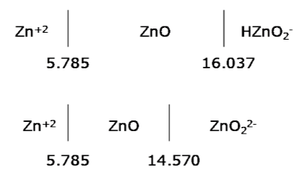
Now we can see that if we raise the pH we will convert ZnO into ZnO22- before we form HZnO2-. Thus the arrangement on the diagram will be Zn+2/ZnO/ZnO22-. *
* In this case one could deduce quite quickly that HZnO2- would not appear on the diagram. Raising the pH from above 5.785 would first form ZnO22- before HZnO2-. This eliminates HZnO2- as a possible dominant species. The method outlined above is useful when there are a larger number of hydrolysis states to sort through.
But, this does not mean that HZnO2- does not exist in the Zn-H2O system with unit solute activities. It simply means that there is no pH where it can ever attain unit activity. Consider the two equations:
\[\mathrm{pH} = 16.037 + \log a_{\ce{HZnO2^-}}\]
from equation [52]
\[\mathrm{pH} = 13.103 - \log\!\left\{a_{\ce{HZnO2^-}}/(a_{\ce{ZnO2^{2-}}}=1)\right\} = 13.103 - \log a_{\ce{HZnO2^-}}\]
from equation [53]
Allowing aHZnO2- to be other than 1 and rearranging these:
\[\log a_{\ce{HZnO2^-}} = \mathrm{pH} - 16.037 \tag{128}
\]
\[\log a_{\ce{HZnO2^-}} = 13.103 - \mathrm{pH}\tag{129}
\]
The former applies to the ZnO/HZnO2- equilibrium and the latter to the
HZnO2-/ZnO22- equilibrium. In the ZnO region aHZnO2- increases as pH increases (equation {1}). In the ZnO22- region aHZnO2- increases as pH decreases (equation {2}). Hence at the ZnO/ZnO22- boundary the activity of HZnO2- is as high as it can get. Any deviation in pH from this point causes a decrease in its activity. Solving the equations indicates that this occurs at pH 14.58. Then,
\[\log a_{\ce{HZnO2^-}} = 14.57 - 16.037 = -1.467 = 13.103 - 14.57\]
and \(\,a_{\ce{HZnO2^-}} = 0.0341.\)
Calculating the Eh Lines
Once the hydrolysis lines are known, start at one corner and work from there. The tentative diagram suggests we need a Zn+2/Zn line:
\begin{align*}
&\ce{Zn^{+2}_{aq} + 2e- = Zn_{s}} \tag{130}\\
&n = 2,\ m = 0\\
&\Delta G^{\circ} = \Delta G_f^{\circ}(\ce{Zn}) - \Delta G_f^{\circ}(\ce{Zn^{+2}}) = 0 - (-147.2) = +147.2\ \text{kJ/mol} \tag{131}
\end{align*}
from the Eh equation,
\[\mathrm{Eh} = -\frac{\Delta G^{\circ}}{nF} - \frac{2.303RT}{nF}\log Q_H - \frac{2.303RT\,m}{nF}\,\mathrm{pH} \tag{132}\]
Q-H = 1/aZn+2, solutes at unit activity
\[\mathrm{Eh} = -\frac{147{,}200}{2 \times 96485} - \frac{2.303 \times 8.314 \times 298.15}{2 \times 96485}\log Q_H - \frac{2.303RT \times 0}{nF}\,\mathrm{pH} \tag{133}\]
\[\mathrm{Eh} = -0.7628 - 0.02958 \log\!\left(\frac{1}{a_{\ce{Zn^{+2}}}}\right) = -0.7628\ \mathrm{V} \tag{134}\]
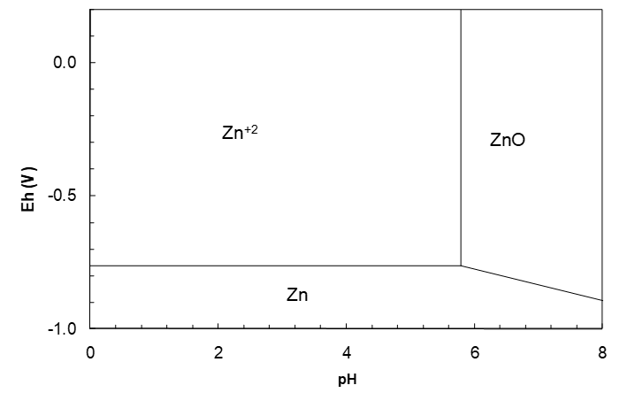
The reduction potential for Zn+2/Zn is a constant, independent of pH. It will be a horizontal line on the Eh-pH diagram. Assume a hypothetical redox couple that will supply electrons. As long as the reduction potential >-0.7628 V, Zn+2 will persist. Once the reduction potential becomes ≤-0.7628 V, Zn+2 is a strong enough oxidant to accept the electrons and be reduced. Thus as we lower the reduction potential we form Zn metal. Hence, as per our tentative diagram (Figure 4.4) the Zn(II) species lie above Zn metal. The line separates the Zn+2 and Zn regions on the diagram. Above the line Zn+2 is predominant; below it Zn is. The line will run from low pH to the pH where the next dominant Zn(II) species occurs, i.e. to pH 5.785. Above that pH ZnO is dominant and not Zn+2. Hence the line stops at pH 5.785.
Next we need the ZnO/Zn couple line. Write the balanced half reaction:
\[
\ce{ZnO = Zn}
\]
\[
\ce{ZnO = Zn + H2O}
\]
\[
\ce{ZnO + 2H^+ = Zn + H2O}
\]
\[
\ce{ZnO_{s} + 2H^+_{aq} + 2e^- = Zn_{s} + H2O_{l}}
\tag{135}
\]
\[
n = 2, \quad m = 2, \quad Q_H = 1
\quad
\text{(there are no solute species; }
2.303RT \log Q_H / nF = 0)
\]
\[
\Delta G^\circ
= \Delta G_f^\circ(\ce{H2O})
- \Delta G_f^\circ(\ce{ZnO})
= -237.15 - (-318.3)
= 81.15\ \text{kJ/mol}
\tag{136}
\]
\[
\mathrm{Eh}
=
-\frac{81{,}150}{2 \times 96{,}485}
-
\frac{2.303RT}{nF}\log 1
-
\frac{2.303 \times 8.314 \times 298.15 \times 2}
{2 \times 96{,}485}
\,\mathrm{pH}
\tag{137}
\]
\[
\mathrm{Eh}
= -0.4205 - 0.05917\,\mathrm{pH}
\tag{138}
\]
Note: at pH 5.785 where the Zn+2/Zn line stops Eh = -0.7628 V, the same value as for the Zn+2/Zn couple. At pH 5.785 and Eh -0.7628 there are three species in equilibrium: Zn+2, ZnO and Zn. The potentials then for the Zn+2/Zn and ZnO/Zn couples must be equal, otherwise there would be a driving force for a reaction (Zn+2 or ZnO) « Zn. This is true in general. The point at which one line stops must be the point where the next starts.* The Zn+2/ZnO vertical line also stops at the same point; Zn(II) species cannot extend into the Zn metal region. The Zn+2/ZnO vertical line runs up from Eh = -0.7628 V to the top of the diagram. The diagram to this point is shown in Figure 4.5.
Consider an erroneous calculation producing the diagram illustrated below. This would imply that we could hydrolyse Zn metal to from ZnO. Clearly that is not possible. Such considerations are another clue that if two adjoining Eh lines do not meet at a point, there has been a calculation error, perhaps of a hydrolysis pH, or of an Eh equation
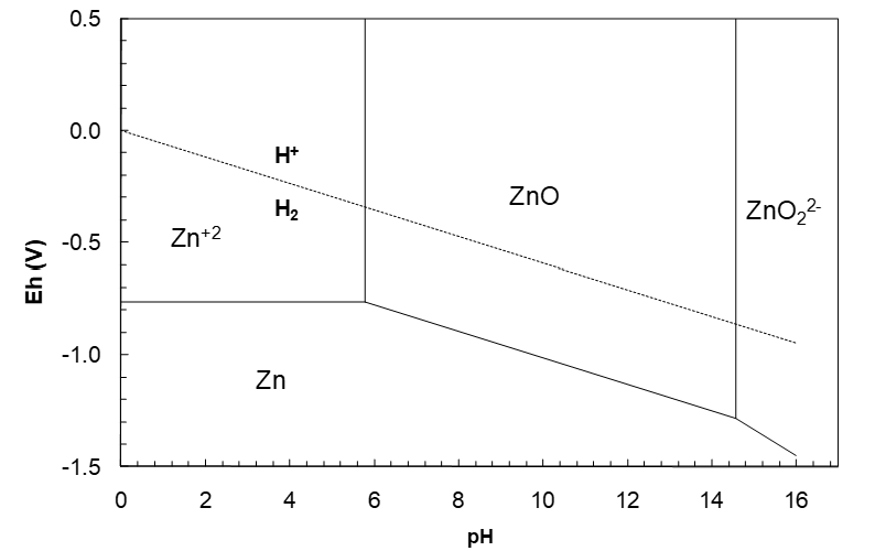
The ZnO/Zn line runs to pH 14.570, beyond which ZnO22- becomes the dominant Zn(II) species. Then we need a ZnO22-/Zn line:
\[\ce{ZnO2^{2-}_{aq} + 4H+_{aq} + 2e- = Zn_{s} + 2H2O_{l}} \tag{139}\]
\[\;n = 2,\ m = 4,\ Q_H = 1/a_{\ce{ZnO2^{2-}}}\]
\[\Delta G^{\circ} = 2\Delta G_f^{\circ}(\ce{H2O}) - \Delta G_f^{\circ}(\ce{ZnO2^{2-}}) = 2 \times (-237.15) - (-389.1) = -85.20\ \text{kJ/mol} \tag{140}\]
\[\mathrm{Eh} = -\frac{85{,}200}{2 \times 96485} - \frac{2.303 \times 8.314 \times 298.15}{2 \times 96485}\log Q_H - \frac{2.303 \times 8.314 \times 298.15 \times 4}{2 \times 96485}\,\mathrm{pH} \tag{141}\]
\[\mathrm{Eh} = 0.4415 - 0.02958 \log\!\left(\frac{1}{a_{\ce{ZnO2^{2-}}}}\right) - 0.1183\,\mathrm{pH} = 0.4415 - 0.1183\,\mathrm{pH} \tag{142}\]
The ZnO/ZnO22- vertical line runs up from the Eh at pH 14.57. The Eh at the point of intersection is easily calculated from the ZnO/Zn or ZnO22-/Zn Eh equations at pH 14.57. Plotting this yields the diagram in Figure 10. Note that the relative slopes of the lines are governed by the ratio m/n. The water Eh lines are included in such diagrams to remind us of the thermodynamic constraints of water stability.
Reading the Diagram
Now that we have the diagram we can start to use it. Zinc oxide is a solid and it is clearly quite highly soluble in dilute acid (pH 5.79 can sustain something on the order of 1 M (unit activity and thus somewhat less than 1 M) of a soluble zinc salt (e.g. ZnSO4). However, by far the most common zinc mineral in nature is sphalerite, ZnS. One way to treat sphalerite is to roast it. The resulting product is ZnO (zinc calcine). This then can be leached in dilute acid. (Usually around pH 4 to improve the reaction rate.*) We can also see from the diagram that leaching ZnO in base is impractical. A pH of >14.6 would be required; probably on the order of 10 M NaOH. Since NaOH is a costly reagent, and there is no simple way to produce Zn metal from such a strongly basic solution, leaching in base is obviated.
*Note that a ZnO s/ZnSO4 aq mixture is a buffer. The vertical lines simply calculate the buffer pH under the specified conditions, in this case, unit activities of solutes. This is true for vertical lines in general (except at very high/low pH where the buffering effect is lessened). Because the ZnO s/ZnSO4 aq mixture is a buffer, it should not permit a pH <5.79. But, since the rate of reaction is only moderate, it takes time for the pH to reach equilibrium. In a leaching situation where slurries are continuously flowing, equilibrium may not be attained. Then it is quite possible to maintain a pH less than the thermodynamic buffer point.)
One of the most common ways of recovering pure metal from aqueous solutions is electrolysis (electrowinning). This forces an otherwise thermo-dynamically unfavourable reduction. However, it is evident from the diagram that at all pH where Zn+2 is dominant, the Zn+2/Zn couple lies far below the H+/H2 line, i.e attempting to reduce Zn+2 in aqueous solution should produce hydrogen gas first; H+ is a much stronger oxidant than Zn+2 at all relevant pH. Nevertheless, Zn+2 electrowinning (EW) is practiced all over the world. This seems paradoxical. It is another case of where kinetics apparently trumps thermodynamics. It turns out that on the surface of very pure zinc metal, reduction of H+ to H2 is very slow, while the rate at which Zn+2 can be reduced to Zn is very fast. Thus in Zn EW most of the electricity goes to plate Zn metal, while a small fraction goes to form H2. The driving force for hydrogen evolution increases as pH decreases (the Eh gap between the H+/H2 and Zn+2/Zn couples increases, meaning that H+ becomes an increasingly stronger oxidant relative to Zn+2.)
The Effects of Varying Ionic Solute Activities
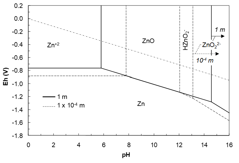
Changing the solute activities will shift the lines where Eh is a function of solute activities. The effects are shown in the Eh-pH diagram in Figure 4.8 (below). At 10-4 m solute activities a region for HZnO2- is present. The Zn+2 region has expanded to lower Eh and higher pH. The lower Eh for Zn+2 reduction occurs due to the –log(1/aZn+2) term. The shift in pH can be rationalized on the basis of the reaction,
\[\ce{ZnO_s + 2H^{+}_{aq} = Zn^{2+}_{aq} + H2O_l} \tag{143}\]
\[\;K = \frac{a_{Zn^{2+}}}{(a_{H^+})^2} \tag{144}\]
If aZn+2 drops, so must aH+, i.e. pH increases. Other changes can be similarly understood. Finally, the ZnO region shrinks with decreasing solute activities, while the ZnO22- region expands.
4.3 The Sulfur-Water Diagram
Sulfur plays a large role in hydrometallurgy (and pyrometallurgy). Many metals of commercial interest occur in sulfide minerals. Hence it is important that we be able to develop and understand the sulfur-water Eh-pH diagram. Once that is in place we can combine it with metal-water diagrams to get information about aqueous chemistry associate with metal sulfides.
Chemical Species and Data
Again, we need species with the elements of sulfur and water (S, H, and O). Sulfur forms a wide range of oxoanions and solid elemental sulfur has three common forms that occur in hydrometallurgy. These are shown in Table 4.2 (below).
| Table 4.2 - The common sulfur-water (S-O-H) compounds and ions and their corresponding sulfur oxidation states. | |||
|---|---|---|---|
| Species | Sulfur Oxidation State | Species | Sulfur Oxidation State |
| H2S g, HS-, S2- | -2 | SxO62-, x ≥ 3 | +10/x |
| H2Sx, HSx-, Sx2-, x = 2–9 1 | 2/x | SO2 aq, HSO3-, SO32- | +4 |
| S8 (rhombohedral most stable; monoclinic stable at 95.3 °C–~119 °C (melting point)) 2 | 0 | S2O62- 6 | +5 |
| S2O32- 3 | 2 | HSO4-, SO42- | +6 |
| S2O42- 4 | 3 | H2S2O8, HS2O8-, S2O82-
H2SO5, HSO5- 7 |
S(+6) and O(-1) |
| 1 Polysulfide; stable only in basic solutions. 2 A polymeric form of sulfur exists that is quite common when elemental sulfur forms around room temperature. It gradually reverts to rhombohedral sulfur. 3 Unstable below pH ~5.5; most stable at pH ~10. 4 Very powerful reductant; only moderately stable; uncommon in hydrometallurgy. 5 Polythionates. Parent acids (H2SxO6) are strong acids; x = 3, 4 moderately stable; x ≥ 5 decompose moderately quickly. 6 Dithionate. Parent acid (H2S2O6) is strong and unstable. 7 Peroxodisulfate and peroxosulfate; powerful oxidants; limited applications in hydrometallurgy. |
|||
The oxidation states can be easily determined by the method outlined earlier in these notes. There are a lot of species to consider. It turns out, however, that only the S(-2), elemental sulfur and S(+6), i.e. sulfate species are thermodynamically stable. Many of the others have substantial kinetic stability (decompose slowly) under certain conditions, but in time they will revert to one of the three stable compounds. What this usually means is that only these three will appear on an Eh-pH diagram that considers the most thermodynamically stable species. The reasons for this will be demonstrated later. (However, because many other sulfur species have kinetic stability, and for other reasons, Eh-pH diagrams can be drawn to include the relevant ones. This requires some additional considerations.) Thermodynamic data for the three sulfur species are given in the table below.
| Table 4.3 - ΔG°f data for the thermodynamically stable S-H2O species at 25°C. | |
|---|---|
| Species | Δ G°f kJ/mol |
| H2Sq | -33.56 |
| H2Saq | -27.83 |
| HS-aq | 11.44 |
| S2-aq | 117* |
| S8 (rhombohedral) | 0 |
| HSO4-aq | -755.91 |
| SO42-aq | -744.55 |
| * There is debate over this value. In hydrometallurgy a value of about 92.2 kJ/mol is commonly accepted, but more recent work suggests that the higher value is probably more accurate. | |
Tentative Diagram
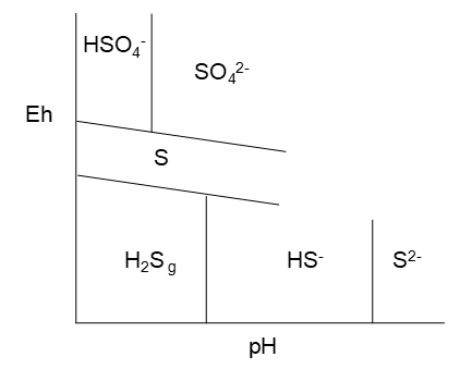
Again, we might expect the most oxidized species to appear at the highest Eh (have the highest reduction potentials). Of the S(+6) species, H2SO4 is a strong acid and fully dissociates into HSO4- and H+. HSO4- is a weak acid. We should expect HSO4- to be dominant at lower pH. Likewise the order for the S(-2) species should be, from low to high pH: H2S, HS-, S2-. Then our diagram should look somewhat like that in Figure 4.9. Based on our experience with the Zn–H2O diagram we might expect negatively Eh sloping lines.
Hydrolysis (Acid Dissociation) Lines
The pH values for the vertical lines can be calculated as before:
Step 1
[latex]\begin{align*} \ce{H2S_g} &= \ce{HS^-_{aq}} + \ce{H+_{aq}} \tag{145} \\ \Delta G^{\circ} &= 11.44 - (-33.56) = 45.00\ \text{kJ/mol} \tag{146} \end{align*}[/latex]
Step 2
[latex]\begin{align*} \ce{HS^-_{aq}} &= \ce{S^{2-}_{aq}} + \ce{H+_{aq}} \tag{147} \\ \Delta G^{\circ} &= 117 - 11.44 = 105.56\ \text{kJ/mol} \tag{148} \end{align*}[/latex]
Step 3
[latex]\begin{align*} \ce{HSO4^-_{aq}} &= \ce{SO4^{2-}_{aq}} + \ce{H+_{aq}} \tag{149} \\ \Delta G^{\circ} &= -744.55 - (-755.91) = 11.36\ \text{kJ/mol} \tag{150} \end{align*}[/latex]
The pH values for the acid dissociation reactions can be calculated next. We will use unit activities for solutes and 1 atm pressure for gases.
Step 1
For H2S/HS- with Q-H = aHS-/PH2S and m = -1 (H+ is a product):
\[\;pH = -\frac{45{,}000}{2.303 \times 8.314 \times 298.15 \times (-1)} - \frac{1}{(-1)}\log\!\left(\frac{a_{HS^-}}{P_{H_2}}\right) \tag{151}\]
\[\;pH = 7.883 + \log\!\left(\frac{a_{HS^-}=1}{P_{H_2}=1}\right) = 7.883 \tag{152}\]
Step 2
For HS-/S2- with Q-H = aS2-/aHS- = 1 (at all activities) and m = -1:
\[\;pH = -\frac{105{,}560}{2.303 \times 8.314 \times 298.15 \times (-1)} = 18.5 \tag{153}\]
Note that because of the form of Q-H, the log term falls away. If we use ΔG°f(S2-) = 92.2 kJ/mol, the pH becomes 14.15. This is quite commonly seen in hydrometallurgy literature, though probably incorrect.
Step 3
For HSO4-/SO42- with Q-H = aSO42-/aHSO4- = 1 at all activities and m = -1:
\[\;pH = -\frac{11{,}360}{2.303 \times 8.314 \times 298.15 \times (-1)} = 1.990 \tag{154}\]
Calculating the Eh Lines
We will start at the lower left and work out from there. First then we need a S-H2S reduction line:
\[\ce{S_s + 2H+_{aq} + 2e^- = H2S_g} \tag{155}\]
\[n = 2,\; m = 2,\; Q_H = P_{H_2S} = 1\]
\[\Delta G^{\circ} = -33.56\ \text{kJ/mol} \tag{156}\]
\[\;E_h = -\frac{-33{,}560}{2 \times 96485} - \frac{2.303 \times 8.314 \times 298.15}{2 \times 96485}\log Q_H - \frac{2.303 \times 8.314 \times 298.15 \times 2}{2 \times 96485}\,pH \tag{157}\]
\[\;E_h = 0.1739 - 0.02958\log P_{H_2S} - 0.05917\,pH \tag{158}\]
\[\;E_h = 0.1739 - 0.05917\,pH \tag{159}\]
This line will run from low pH up to the H2S/HS- vertical line at pH 7.883. Beyond that point H2S is no longer dominant; HS- is. Hence we need a S/HS- line:
\[\ce{S_s + H+_{aq} + 2e- = HS^-_{aq}} \tag{160}\]
\[\text{n = 2, m = 1, } Q_H = a_{\ce{HS^-}} = 1\]
\[\Delta G^\circ = 11.44\ \text{kJ/mol} \tag{161}\]
\[
E_h
= -\frac{11{,}440}{2 \times 96485}
- \frac{2.303 \times 8.314 \times 298.15}{2 \times 96485}\log Q_H
- \frac{2.303 \times 8.314 \times 298.15 \times 1}{2 \times 96485}\,pH
\tag{162}
\]
\[
E_h = -0.05928 - 0.02958 \log(a_{\ce{HS^-}}) - 0.02958\,pH
\tag{163}
\]
\[
E_h = -0.05928 - 0.02958\,pH
\tag{164}
\]
This line starts at pH 7.883. The diagram to this point is shown in Figure 4.10 (below). At this point it is a good idea to begin to work up as well. (Looking at the diagram so far we might expect that an HSO4-/S line could intersect the S/HS- line.) Thus we need an HSO4-/S line next.
\[\ce{HSO4^-_{aq} + 7H+ + 6e^- = S_s + 4H2O_l} \tag{165}\]
\[n = 6,\ m = 7,\ Q_H = 1/a_{HSO4^-} = 1\]
\[\Delta G^{\circ} = 4 \times (-237.15) - (-755.91) = -192.69\ \text{kJ/mol} \tag{166}\]
\[\;E_h = -\frac{-192{,}690}{6 \times 96485} - \frac{2.303x8.314x298.15}{6 \times 96485}\log Q_H - \frac{2.303x8.314x298.15 \times 7}{6 \times 96485}\,pH \tag{167}\]
\[\;E_h = 0.3329 - 0.009861\log\!\left(\frac{1}{a_{HSO4^-}}\right) - 0.06903\,pH \tag{168}\]
\[\;E_h = 0.3329 - 0.06903\,pH \tag{169}\]
This line runs from low pH to pH 1.990, after which SO42- becomes dominant. Next we need the SO42-/S line.
\[\ce{SO4^{2-}_{aq} + 8H+ + 6e^- = S_s + 4H2O_l} \tag{170}\]
\[n = 6,\ m = 8,\ Q_H = 1/a_{SO4^{2-}} = 1\]
\[\Delta G^{\circ} = 4 \times (-237.15) - (-744.55) = -204.05\ \text{kJ/mol} \tag{171}\]
\[\;E_h = -\frac{-204{,}050}{6 \times 96485} - \frac{2.303x8.314x298.15}{6 \times 96485}\log Q_H - \frac{2.303x8.314x298.15 \times 8}{6 \times 96485}\,pH \tag{172}\]
\[\;E_h = 0.3525 - 0.009861\log\!\left(\frac{1}{a_{SO4^{2-}}}\right) - 0.07889\,pH \tag{173}\]
\[\;E_h = 0.3525 - 0.07889\,pH \tag{174}\]
This line begins at pH 1.990. Plotting the two new lines yields the diagram below. It is apparent that the SO42-/S and S/HS- lines intersect. Where the lines meet is where they stop. Continuing the lines past their point of intersection makes no sense as shown in Figure 4.11 (below). This would create apparent regions with more than one S species as dominant. The pH and Eh of intersection need to be calculated using the Eh equations so that the point of intersection can be plotted.
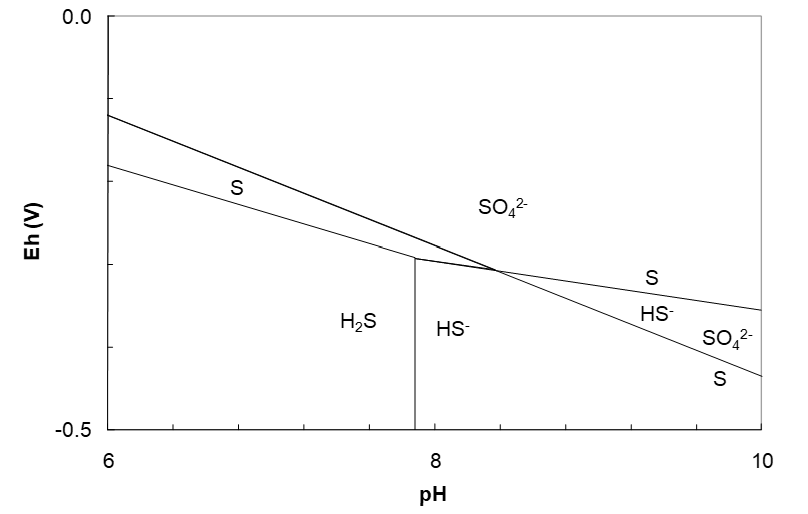
The relevant equations are:
\[\text{S/HS:}\quad E_h = -0.05928 - 0.02958\,pH \tag{175}\]
\[\text{SO}_4^{2-}\text{/S:}\quad E_h = 0.3525 - 0.07889\,pH \tag{176}\]
Solving these two equations gives the pH, Eh point = 8.351, -0.3063 V.
Looking at the diagram to this point, it appears that we have a SO42- region and a HS- region yet that need a boundary. This calls for a SO42-/HS- line.
\[\ce{SO4^{2-}_{aq} + 9H+ + 8e^- = HS^-_{aq} + 4H2O_l} \tag{177}\]
\[n = 8,\ m = 9,\ Q_H = a_{HS^-}/a_{SO4^{2-}} = 1\ (\text{regardless of solute activities})\]
\[\Delta G^{\circ} = 4 x (-237.15) + 11.44 - (-744.55) = -192.61\ \text{kJ/mol} \tag{178}\]
\[\;E_h = -\frac{192610}{8 x 96485} - \frac{2.303x8.314x298.15}{8 x 96485}\log Q_H - \frac{2.303x8.314x298.15 x 9}{8 x 96485}\,pH \tag{179}\]
\[\;E_h = 0.2495 - 0.06656\,pH \tag{180}\]
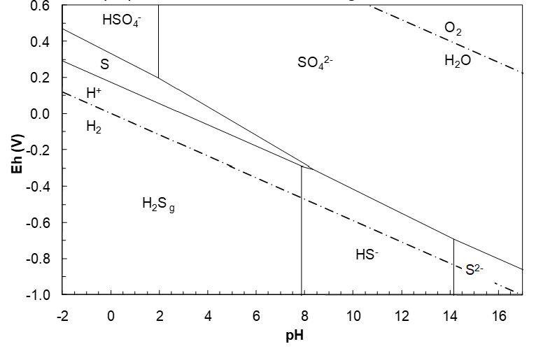
This line starts at pH 8.351 and would run to the HS-/S2- line at pH 18.5. However, such extremely high pH (on the order of 30,000 M OH-) is not attainable. (A pH of 14 corresponds to ~ 1 M OH-). Next we could calculate a SO42-/S2- line, though it is of little significance since the pH involved is so unrealistically high. However, if one takes ΔG°f(S2-) to be 92.2 kJ/mol (as is common in the hydrometallurgical literature) then the HS-/S2- pH would be 14.14 and a SO42-/S2- line would be reasonable. The half reaction is:
\[\ce{SO4^{2-}_{aq} + 8H+_{aq} + 8e^- = S^{2-}_{aq} + 4H2O_l} \tag{181}\]
\[n = 8,\ m = 8,\ Q_H = a_{S^{2-}}/a_{SO4^{2-}} = 1\ (\text{regardless of solute activities})\]
\[\Delta G^{\circ} = 4 x (-237.15) + 92.2 - (-744.55) = -111.85\ \text{kJ/mol} \tag{182}\]
(IF we take ΔG°f(S2-) to be to the conventional value of 92.2 kJ/mol, rather than the more likely 117 kJ/mol.)
\[\;E_h = -\frac{111{,}850}{8 x 96485} - \frac{2.303x8.314x298.15}{8 x 96485}\log Q_H - \frac{2.303x8.314x298.15 x 8}{8 x 96485}\,pH \tag{183}\]
\[\;E_h = 0.1449 - 0.05917\,pH \tag{184}\]
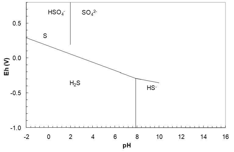
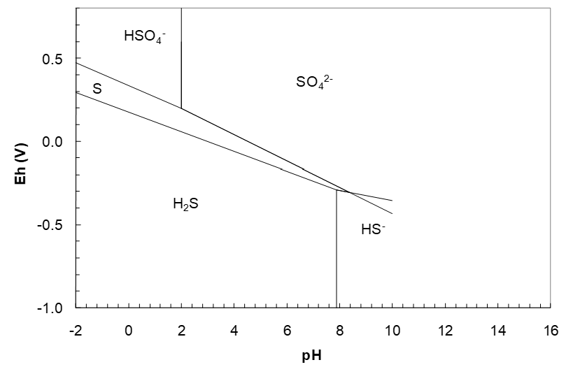
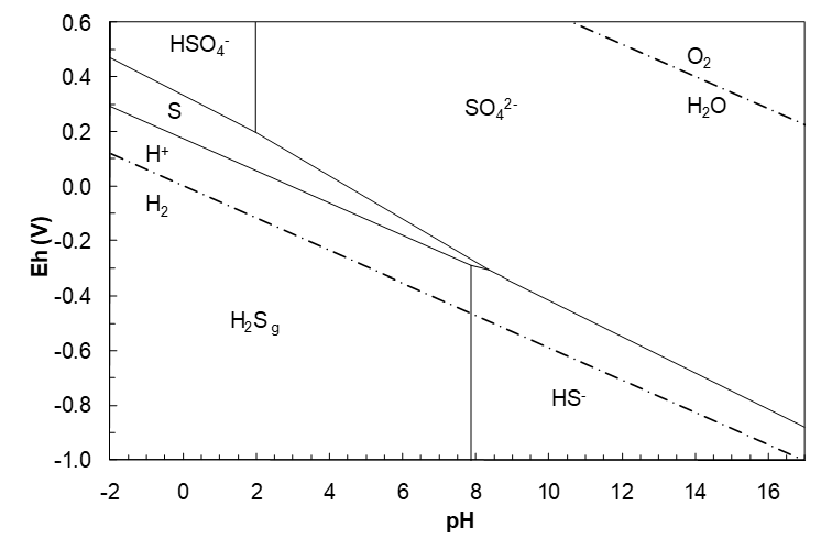
The final diagrams are shown in Figure 4.12 and Figure 4.13 (below). The sulfur region is a downward sloping wedge that is thermodynamically stable to about pH 8.4. This influences the shape of many metal sulfide regions in corresponding Eh-pH diagrams (in many cases the metal sulfide region parallels the sulfur region). Changing the activities of the solutes or the gas pressure will change the diagram.
Less Stable S-H2O Species
We stated earlier that only S(-2), S and S(+6) species would appear on the diagram. Here we will see why that is so. Consider thiosulfate, S2O32-, ΔG°f = -532.21 kJ/mol. The S oxidation state is +2. We might expect that a region for S2O32- would lie above the S region and below the SO42- region. Plausible half reactions and Eh equations (solute activities = 1) are shown below.
Step 1
\[\mathrm{SO_4^{2-}\ to\ S_2O_3^{2-}:}\]
\[\ce{2SO4^{2-}_{aq} + 10H+_{aq} + 8e^- = S2O3^{2-}_{aq} + 5H2O_l} \tag{185}\]
\[n = 8,\ m = 10,\ Q_H = a_{S2O3^{2-}}/(a_{SO4^{2-}})^2 = 1\]
\[\Delta G^{\circ} = 5 x (-237.15) + (-532.21) - 2 x (-744.55) = -228.86\ \text{kJ/mol} \tag{186}\]
\[\;E_h = -\frac{228{,}860}{8 x 96485} - \frac{2.303x8.314x298.15}{8 x 96485}\log Q_H - \frac{2.303x8.314x298.15 x 10}{8 x 96485}\,pH \tag{187}\]
\[\;E_h = 0.2965 - 0.007396\log\!\left(\frac{a_{S2O3^{2-}}}{(a_{SO4^{2-}})^2}\right) - 0.07396\,pH \tag{188}\]
\[\;E_h = 0.2965 - 0.07396\,pH \tag{189}\]
Step 2
S2O32- to S:
\[\ce{S2O3^{2-}_{aq} + 6H+_{aq} + 4e^- = 2S_s + 3H2O_l} \tag{190}\]
\[n = 4,\ m = 6,\ Q_H = 1/a_{S2O3^{2-}} = 1\]
\[\Delta G^{\circ} = 3 x (-237.15) - (-532.21) = -179.24\ \text{kJ/mol} \tag{191}\]
\[\;E_h = -\frac{179{,}240}{4 x 96485} - \frac{2.303x8.314x298.15}{4 x 96485}\log Q_H - \frac{2.303x8.314x298.15 x 6}{4 x 96485}\,pH \tag{192}\]
\[\;E_h = 0.4644 - 0.01479\log\!\left(\frac{1}{a_{S2O3^{2-}}}\right) - 0.08875\,pH \tag{193}\]
\[\;E_h = 0.4644 - 0.08875\,pH \tag{194}\]
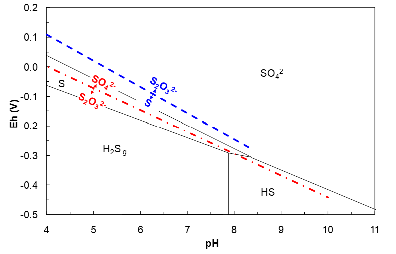
These equations can be plotted on the Eh–pH diagram as shown in Figure 4.15 (below). The diagram shows that the SO42-/S2O32- line occurs within the S region, or within the HS- region. So, if we had SO42- and lowered the reduction potential, we would form the more reduced elemental S before we would form S2O32-. Or, S forms more easily (at higher potential) than does S2O32-. This shows that there cannot be a SO42-/S2O32- line. Similarly, at higher pH, we would form HS- by reduction of SO42- before we form S2O32-. The S2O32-/S line lies above the S region and in the SO42- region. Since S is not stable at this Eh (SO42- is), this line is not possible either. These kinds of considerations would pertain to all the other sulfur species under these conditions, leaving S(-2), S and S(+6) species as the only possibilities to include on the diagram.
Kinetic Effects
The fact that other sulfur species don’t show up on the diagram does not mean they are unimportant. Indeed, thiosulfate is being studied intensively as a complexing agent for gold leaching, and SO2 aq/HSO3-/SO32- are important in some aspects of hydrometallurgy, etc. These species are not stable relative to S(-2), S and S(+6). This means that they will eventually decompose into more stable species by reactions with acid, base or oxygen, or they will disproportionate, e.g.
\[\ce{S2O3^{2-}_{aq} + H+_{aq} = S_s + HSO3^-_{aq}} \tag{195}\]
However, they have significant kinetic stability and under suitable conditions will persist for long enough times to be of use in chemical processing. Then an Eh-pH diagram involving such species may be of interest. One way to draw such a diagram is to leave out one or more of the more stable species. To draw an Eh-pH diagram that also includes thiosulfate one could leave out sulfate. Then lines for other sulfur species like S2O32-, SxO62-, etc. can be drawn and will yield reasonable diagrams. This is not unreasonable; the conversion of intermediate oxidation state sulfur species into sulfate is quite slow under some conditions.
For oxidation of elemental sulfur to sulfate to occur at a reasonable rate, much stronger oxidants are required than the Eh-pH diagram of Figure 4.14 would suggest. At pH 0 the thermodynamic reduction potential for HSO4- to form S is 0.33 V. Ferric ion (E° = +0.68 V) is not a strong enough oxidant to oxidize sulfur. However, nitrous acid (HNO2) is readily able to oxidize sulfur to HSO4-:
\[\ce{HNO2_{aq} + H+_{aq} + e- = NO_{g} + H2O_l} \quad E^\circ = 0.95\ \text{V} \tag{196}\]
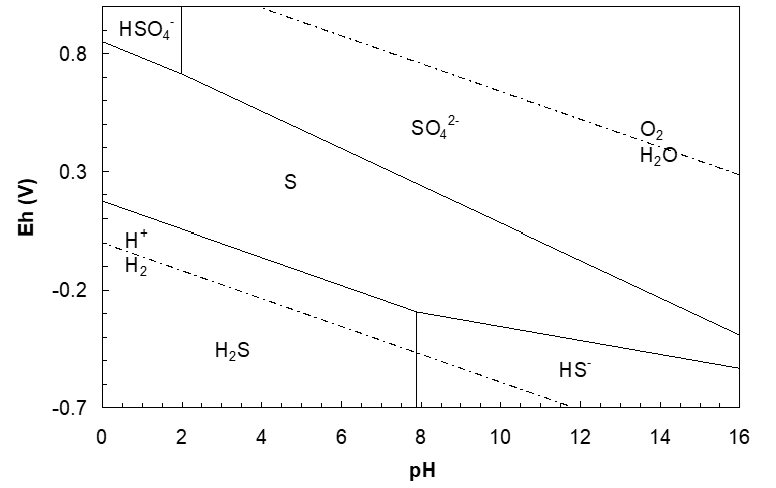
These observations reflect the fact that sulfur is kinetically extremely stable, much more so than the thermodynamics suggests. This does not mean that thermodynamics is wrong, just that the reactions are exceedingly slow. One can take this kinetic stability into account and construct a diagram which reflects it. Adding 300 kJ/mol to ΔG°f(SO42-) adjusts it to -445 kJ/mol and adjusts ΔG°f(HSO4-) to 456 kJ/mol (compared to the data in Table 4.1). This raises the HSO4-/S and the SO42-/S lines significantly. E° for HSO4-/S then (at pH = 0) becomes +0.85 V. This is closer to the experimental evidence that suitably strong oxidants can oxidize sulfur, overcoming its kinetic stability. The adjusted S-H2O diagram is shown below. It must be stressed that this is not thermodynamically correct. But, it might be of some use when trying to rationalize kinetic factors.
4.4 The Zn-S-H2O Eh-pH diagram
Metal sulfides play an important role in hydrometallurgy. Understanding their leaching chemistry requires an understanding of the associated thermodynamics. Now that we have the Zn-H2O and S-H2O diagrams we can draw the Zn-S-H2O diagram. And, we do need both of these preceding diagrams to do this. That we are considering the Zn-S-H2O system requires that we consider all species that are composed of the elements Zn, S, H and O. This adds only one new species in this case:
\[\ce{ZnS},\ \text{with a }\Delta G_f^{\circ}\text{ of }-198.3\ \text{kJ/mol}\]
Our task is to determine the extent of the ZnS region of stability under the given conditions (unit activities for solutes; molal scale, 25°C and 1 atm pressure).
Determining if Hydrolysis Reactions Occur
We need first to know what sorts of species ZnS hydrolysis can produce. Thus we need to know the oxidation states of Zn and S. We know that Zn can have two oxidation states: +2 and 0. And we know that S can have two oxidation states (as S alone, not sulfur oxyanions or polysulfides): -2 and 0. The 0 oxidation state does not make sense for a compound; then we would have a mixture of elemental S and elemental Zn. (ΔG°f is a substantial negative number. Hence ZnS is a stable compound and not a mixture of elements.) This leaves Zn(+2) and S(-2). Therefore, hydrolysis reactions must form Zn(+2) and S(-2) species, otherwise electron transfers will occur. The only possible Zn(+2) species are Zn2+, ZnO and ZnO22-. The possible S(-2) species are H2S, HS- and perhaps S2- (in principle). The next question is what combinations of Zn(+2) and S(-2) species are possible? To answer that question we first overlay the Zn-H2O and S-H2O diagrams, as shown in Figure 4.16 (below). This diagram tells us what Zn(+2) and S(-2) species can co-exist in the same region.
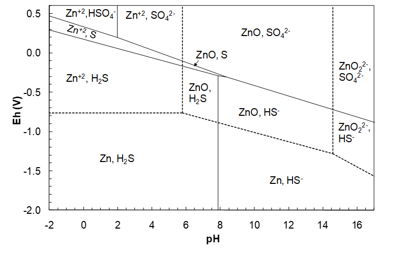
(We already saw that this was possible when we drew the Zn-H2O diagram. We determined that various Zn species and water could co-exist within specified domains of Eh-pH conditions. Thus it should not come as a surprise that species of different chemical elements can co-exist. And we know this from experience. There are lots of thermodynamically stable compounds of different elements that can be dissolved in an aqueous solution.) Looking at the diagram above we see that the following Zn(+2) and S(-2) species can co-exist (they have overlapping regions):
\[\ce{Zn^{2+}},\ \ce{H2S}\]
\[\ce{ZnO},\ \ce{H2S}\]
\[\ce{ZnO},\ \ce{HS^-}\]
\[\ce{ZnO2^{2-}},\ \ce{HS^-}\]
If we included a region for S2-, as per Figure 4.16 we would also see that ZnO22- and S2- have a region of overlap.
The next step is to write hydrolysis reactions that involve these pairs of Zn and S species and ZnS, then calculate pH values for the reactions and see if they can be plotted on the diagram, i.e., do any of them make sense? Reactions are shown below. Start with ZnS and write the various combinations of Zn(+2) and S(-2) species as products, then balance the reactions. The process is quite simple as the first case below illustrates.
Step 1
\[\ce{ZnS} = \ce{Zn^{2+}} + \ce{H2S}\]
\[\ce{ZnS_s} + \ce{2H+_{aq}} = \ce{Zn^{2+}_{aq}} + \ce{H2S_{aq}} \tag{197}\]
\[\Delta G^\circ = -33.56 + (-147.2) - (-198.3) = 17.54\ \text{kJ/mol} \tag{198}\]
Step 2
\[\ce{ZnS_s} + \ce{H2O_l} = \ce{ZnO_s} + \ce{H2S_g} \tag{199}\]
\[\Delta G^\circ = -33.56 + (-318.3) - (-237.15) - (-198.3) = 83.59\ \text{kJ/mol} \tag{200}\]
Step 3
\[\ce{ZnS_s} + \ce{H2O_l} = \ce{ZnO_s} + \ce{HS^-_{aq}} + \ce{H^+_{aq}} \tag{201}\]
\[\Delta G^\circ = 11.44 + (-318.3) - (-237.15) - (-198.3) = 128.59\ \text{kJ/mol} \tag{202}\]
Step 4
\[\ce{ZnS_s} + \ce{2H2O_l} = \ce{ZnO2^{2-}_{aq}} + \ce{HS^-_{aq}} + \ce{3H^+_{aq}} \tag{203}\]
\[\Delta G^\circ = 11.44 + (-389.1) - 2(-237.15) - (-198.3) = 294.94\ \text{kJ/mol} \tag{204}\]
Step 1
For ZnS/Zn+2,H2S with Q-H = PH2S aZn+2 and m = 2:
\[\mathrm{pH}=-\frac{17540}{2.303\times8.314\times298.15\times2}-\frac{1}{2}\log\!\left(P_{\ce{H2S}}a_{\ce{Zn^{2+}}}\right)\tag{205}\]
\[\mathrm{pH}=-1.536+0.5\log\!\left(P_{\ce{H2S}}a_{\ce{Zn^{2+}}}\right)=-1.536\tag{206}\]
Step 2
For ZnS/ZnO,H2S, m= 0, n = 0 so this reaction cannot be depicted on an Eh-pH diagram (it is both Eh- and pH-independent).
Step 3
For ZnS/ZnO,HS-, with Q-H = aHS- and m = -1 (H+ is a product):
\[\mathrm{pH}=-\frac{128590}{2.303\times8.314\times298.15\times(-1)}-\frac{1}{(-1)}\log a_{\ce{HS^-}}\tag{207}\]
\[\mathrm{pH}=22.53+\log a_{\ce{HS^-}}=22.525\tag{208}\]
Step 4
For ZnS/ZnO22-,HS-, with Q-H = aHS- aZnO22- and m = -3:
\[\mathrm{pH}=-\frac{294940}{2.303\times8.314\times298.15\times(-3)}-\frac{1}{(-3)}\log\!\left(a_{\ce{HS^-}}\,a_{\ce{ZnO2^{2-}}}\right)\tag{209} \]
\[\mathrm{pH}=17.22+\log\!\left(a_{\ce{HS^-}}\,a_{\ce{ZnO2^{2-}}}\right)=17.222\tag{210}\]
The pH for the first reaction is -1.536. (Recall that this is the pH where all species have the specified activities.) This is very low, but not unattainable; concentrated MgCl2/HCl solutions can attain very low pH. The pH value does lie within a region where both Zn2+ and H2S can co-exist (Figure 4.16). Hence this is a plausible hydrolysis reaction. Reaction (199) is not a possible reaction for a ZnS/Zn(+2), S(-2) hydrolysis boundary, as explained above. For reaction (200) the hydrolysis pH is 22.525, which is much too high to be attainable in the first place, and secondly ZnO is not dominant at that pH (nor is HS-; pH for the HS-/S2- buffer point is 18.5). This is not a possible hydrolytic boundary for ZnS either. Finally, reaction (203) has a buffer pH of 17.222. Both ZnO22- and HS- can co-exist at that pH, in principle, although it is extremely high and probably of little practical use. In principle it is a valid hydrolytic boundary, but we will not plot out to that high pH.
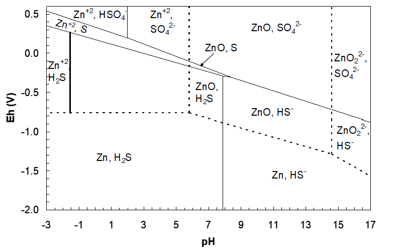
We start with the ZnS/Zn2+, H2S vertical line and plot that, then begin to build the ZnS region. Referring to Figure 4.16, the line will extend through the overlapped region where both Zn2+ and H2S co-exist; form the Zn2+/Zn horizontal line up to the S/H2S line. This is depicted in Figure 4.18 (below).
Note that reaction (203) involves H+ as a product, while in reaction (197) H+ is a reactant. This indicates the difference between the right and left side vertical boundaries. Consider reaction (197): starting with ZnS, lower the pH (add H+ as a reactant) and form Zn2+ + H2S. This indicates that ZnS is on the right of the boundary and Zn2+ + H2S are on the left. Now refer to reaction (203): starting with ZnO22- and HS- and lowering the pH we form ZnS. This indicates that ZnO22- + HS- are on the right of the vertical line while ZnS is on the left. With this line in place the rest of the ZnS region can be drawn.
Eh Lines
From where the vertical line starts (at low Eh), we see that we need a line to separate ZnS and the Zn, H2S line; a ZnS/Zn, H2S line. (We cannot have a ZnS/Zn2+, H2S line; we just drew that and it was a vertical line). We need a reduction half reaction. A lower boundary line should reduce ZnS to form products with lower oxidation state. Since we start in the Zn2+, H2S region, the only thing that can be reduced is Zn(+2), in ZnS, to form Zn and H2S. The half reaction is:
\[\ce{ZnS = Zn + H2S}\]
\[\ce{ZnS + 2H+ = Zn + H2S}\]
\[\ce{ZnS_s + 2H+_{aq} + 2e- = Zn_s + H2S_g}\]
\[\text{n = 2, m = 2, }Q_H = P_{\ce{H2S}}\]
\[\Delta G^{\circ} = -33.56 - (-198.3) = 164.74\ \text{kJ/mol}\tag{211}\]
\[E_h=-\frac{164{,}740}{2\times96485}-\frac{2.303\times8.314\times298.15}{2\times96485}\log Q_H-\frac{2.303\times8.314\times298.15\times2}{2\times96485}pH\tag{212}\]
\[E_h=-0.8537-0.02958\log P_{\ce{H2S}}-0.05917pH\tag{213}\]
\[E_h=-0.8537-0.05917pH \]
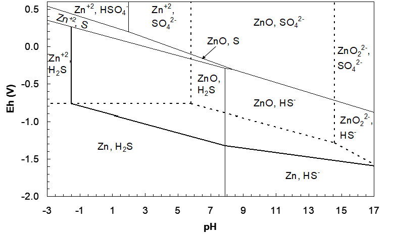
This line will extend from the vertical line at pH -1.536 and to the H2S/HS- boundary (pH 7.883), beyond which HS- is dominant, and not H2S. The next line we need then is for ZnS reduction to Zn and HS-.
\[\ce{ZnS}= \ce{Zn}+\ce{HS^-}\]
\[\ce{ZnS}+ \ce{H+}= \ce{Zn}+ \ce{HS^-}\]
\[\ce{ZnS_s}+ \ce{H+_{aq}}+ \ce{2e-}= \ce{Zn_s}+ \ce{HS^-_{aq}}\tag{214}\]
\[\mathrm{n}=2,\ \mathrm{m}=1,\ Q_H=a_{\ce{HS^-}}\]
\[\Delta G^\circ=11.44-(-198.3)=209.74\ \text{kJ/mol}\tag{215}\]
\[\mathrm{E_h}=-\frac{209{,}740}{2\times96485}-\frac{2.303\times8.314\times298.15}{2\times96485}\log Q_H-\frac{2.303\times8.314\times298.15\times1}{2\times96485}pH\tag{216}\]
\[\mathrm{E_h}=-1.087-0.02958\log a_{\ce{HS^-}}-0.02958pH\tag{217}\]
\[\mathrm{E_h}=-1.087-0.02958pH\tag{218}\]
This line begins at pH 7.883 and will run through the overlapped region where both HS- and Zn can co-exist until it intersects the ZnO22-/Zn line. The point of intersection would be 17.22, the vertical line where the ZnS region ends as per equation (210). This could be verified by calculating the pH of intersection of the ZnS/Zn, HS- line (Eh = -1.087 - 0.02958pH) with the ZnO22-/Zn line (Eh = 0.4415 - 0.1183pH) and comparing this with the pH we calculated for the right-side vertical boundary for the ZnS region (equation (210)). However, since the diagram extends to just pH 17, the line will stop at pH 17. The diagram to this point is shown in Figure 4.18 below.
Now the upper boundary can be drawn. We start at the top of the vertical line on the left. We will need a line that runs through the Zn2+, S region. For the lower lines we reduced ZnS to form Zn and H2S or HS-. Now we need to write reduction half reactions of Zn and S species to form ZnS. Since we start in the Zn2+, S region, begin with these species:
\[\ce{Zn^{2+}}+\ce{S}=\ce{ZnS}\]
\[\ce{Zn^{2+}_{aq}}+\ce{S_s}+\ce{2e-}=\ce{ZnS_s}\tag{219}\]
\[\mathrm{n}=2,\ \mathrm{m}=0\ (\text{a flat line}),\ Q_H=\frac{1}{a_{\ce{Zn^{2+}}}}\]
\[\Delta G^\circ=-198.3-(-147.2)=-51.1\ \text{kJ/mol}\tag{220}\]
\[\mathrm{E_h}=-\frac{51{,}100}{2\times96485}-\frac{2.303\times8.314\times298.15}{2\times96485}\log Q_H\tag{221}\]
\[\mathrm{E_h}=0.2648-0.02958\log a_{\ce{Zn^{2+}}}=0.2648\tag{222}\]
This line will run through the Zn2+, S region until it intersects the HSO4-/S line. The pH of intersection has to be calculated from the equations for the relevant lines (Zn2+, S/ZnS and HSO4-/S). The Eh functions are given by equation (222) and equation (169), respectively:
\[E_h=0.3329-0.06903pH=0.2648\tag{223}\]
Solving gives pH = 0.987. The new line then extends to this pH. Continuing to higher pH past the HSO4-/S line, it enters the HSO4-, Zn2+ overlapped region. Hence now we need a line for reduction of Zn2+ and HSO4- to form ZnS:
\[\ce{Zn^{2+}}+\ce{HSO4^-}=\ce{ZnS}\]
\[\ce{Zn^{2+}}+\ce{HSO4^-}=\ce{ZnS}+ \ce{4H2O}\]
\[\ce{Zn^{2+}}+\ce{HSO4^-}+ \ce{7H+}=\ce{ZnS}+ \ce{4H2O}\]
\[\ce{Zn^{2+}_{aq}}+\ce{HSO4^-_{aq}}+\ce{7H+_{aq}}+\ce{8e-}=\ce{ZnS_s}+ \ce{4H2O_l}\tag{224}\]
\[\mathrm{n}=8,\ \mathrm{m}=7,\ Q_H=\frac{1}{a_{\ce{HSO4^-}}\,a_{\ce{Zn^{2+}}}}\]
\[\Delta G^\circ=4\times(-237.15)+(-198.3)-(-147.2)-(-755.91)=-243.79\ \text{kJ/mol}\tag{225}\]
\[\mathrm{E_h}=-\frac{243{,}790}{8\times96485}-\frac{2.303\times8.314\times298.15}{8\times96485}\log Q_H-\frac{2.303\times8.314\times298.15\times7}{8\times96485}pH\tag{226}\]
\[\mathrm{E_h}=0.3158-0.007396\log\!\left(\frac{1}{a_{\ce{HSO4^-}}\,a_{\ce{Zn^{2+}}}}\right)-0.05177pH\tag{227}\]
\[\mathrm{E_h}=0.3158-0.05177pH\tag{228}\]
When this line is plotted it starts where the previous one left off and intersects with the HSO4-/SO42- line, i.e. at pH 1.990. The developing Eh-pH diagram is shown in the figure below. The latest line is very short. Care is needed to watch for these short lines in other Eh-pH diagrams.
Next we can expect that we will need a Zn+2, SO42-/ZnS line:
\[\ce{Zn^{2+}}+\ce{SO4^{2-}}=\ce{ZnS}\]
\[\ce{Zn^{2+}}+\ce{SO4^{2-}}=\ce{ZnS}+ \ce{4H2O}\]
\[\ce{Zn^{2+}}+\ce{SO4^{2-}}+\ce{8H+}=\ce{ZnS}+ \ce{4H2O}\]
\[\ce{Zn^{2+}_{aq}}+\ce{SO4^{2-}_{aq}}+\ce{8H+_{aq}}+\ce{8e-}=\ce{ZnS_s}+ \ce{4H2O_l}\tag{229}\]
\[\mathrm{n}=8,\ \mathrm{m}=8,\ Q_H=\frac{1}{a_{\ce{SO4^{2-}}}\,a_{\ce{Zn^{2+}}}}\]
\[\Delta G^\circ=4\times(-237.15)+(-198.3)-(-147.2)-(-744.55)=-255.15\ \text{kJ/mol}\tag{230}\]
\[E_h=-\frac{255{,}150}{8\times96485}-\frac{2.303\times8.314\times298.15}{8\times96485}\log Q_H-\frac{2.303\times8.314\times298.15\times8}{8\times96485}pH\tag{231}\]
\[E_h=0.3306-0.007396\log\!\left(\frac{1}{a_{\ce{SO4^{2-}}}\,a_{\ce{Zn^{2+}}}}\right)-0.05917pH\tag{232}\]
\[E_h=0.3306-0.05917pH\tag{233}\]
This line will run through the Zn+2, SO42- overlapped region and stop at the Zn+2/ZnO line (pH 5.785). Next we need a ZnO, SO42-/ZnS line:
\[\ce{ZnO}+\ce{SO4^{2-}}=\ce{ZnS}\]
\[\ce{ZnO}+\ce{SO4^{2-}}=\ce{ZnS}+ \ce{5H2O}\]
\[\ce{ZnO}+\ce{SO4^{2-}}+\ce{10H+}=\ce{ZnS}+ \ce{5H2O}\]
\[\ce{ZnO_s}+\ce{SO4^{2-}_{aq}}+\ce{10H+_{aq}}+\ce{8e-}=\ce{ZnS_s}+ \ce{5H2O_l}\tag{234}\]
\[\mathrm{n}=8,\ \mathrm{m}=10,\ Q_H=\frac{1}{a_{\ce{SO4^{2-}}}}\]
\[\Delta G^\circ=5\times(-237.15)+(-198.3)-(-318.3)-(-744.55)=-321.2\ \text{kJ/mol}\tag{235}\]
\[\mathrm{E_h}=-\frac{321{,}200}{8\times96485}-\frac{2.303\times8.314\times298.15}{8\times96485}\log Q_H-\frac{2.303\times8.314\times298.15\times10}{8\times96485}pH\tag{236}\]
\[\mathrm{E_h}=0.4161-0.007396\log\!\left(\frac{1}{a_{\ce{SO4^{2-}}}}\right)-0.07396pH\tag{237}\]
\[\mathrm{E_h}=0.4161-0.07396pH\tag{238}\]
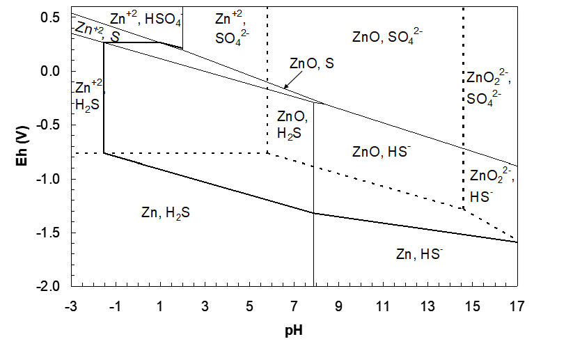
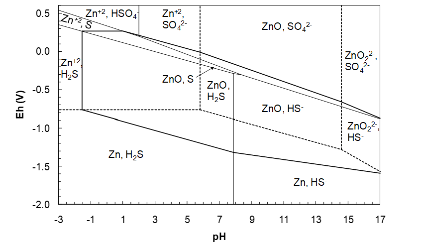
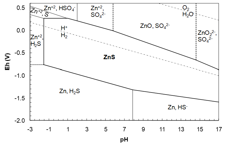
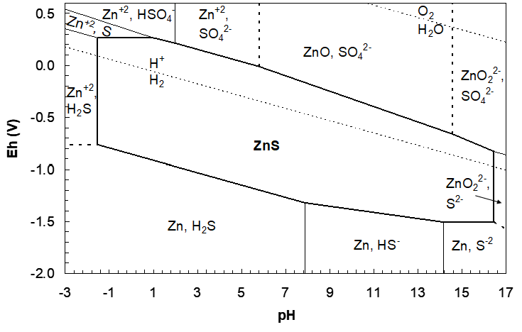
This line runs from pH 14.570 to the upper pH boundary, pH 17. (If we let it continue it would stop at pH 17.22, corresponding to the ZnS/ZnO22-, HS- vertical boundary.) The diagram to this point is shown in Figure 4.21 (below). This completes all boundaries for the ZnS region between pH -1.536 and 17. No high-pH vertical boundary was drawn since it occurs at pH 17.22, beyond the upper limit on this diagram. Upper and lower pH and Eh limits are arbitrary. It depends on what the user wants. However, as mentioned before, a pH of 17 is probably not realistic. The final diagram can be presented in one of two ways. All lines within the ZnS region can be removed, or they can be left in place, usually in a less prominent format. The latter case shows the various pH–Eh regions where ZnS co-exists with either one of a sulfur species or one of a zinc species (but not both; that would violate the principles upon which the diagram is based. Within the ZnS region any Zn species + S species react to form ZnS.) The final diagram with lines inside the ZnS region removed is shown in Figure 25 (again, ΔG°f(S2-) = 117 kJ/mol). Figure 4.22 then shows the alternative diagram where ΔG°f(S2-) = 92.2 kJ/mol.
Note on Setting Activities
Activities of solutes (usually ions, but not always) and pressures of gases are set on the basis of what the user is interested in. In leaching this might vary from about 0.1 m up to about 1 m, simply because we want to have fairly concentrated solutions for efficient processing. In corrosion it might vary greatly, depending on the solutions involved, and so on. In the preceding Zn-S-H2O diagram we set both the Zn solutes and S solutes to have unit activity. However, there is no reason why these cannot differ, and there may be good practical reasons. For instance, we might leach an ore with something on the order of 0.5 m sulfate-containing solution, and generate a copper solution with about 0.02 m copper solute activities.
Activity is a kind of effective concentration. Because aqueous solutions of salts are highly non-ideal, the solutes and the solvent interact strongly. This may make the solute less potentially available to participate in chemical reactions; it is as if its concentration is lower than it actually is. At very low concentrations (<0.001 M for salts of singly charged ions; lower concentration still for more highly charged ions) the solutions can be treated as if almost ideal. But, as concentration increases, the activity decreases, very roughly up to about 1 m.
Beyond this the activity begins to rise again as the amount of water available to interact with the ions starts to decrease. For solutes that can achieve very high solubility in water (e.g. some chloride and nitrate salts) the activity may even greatly exceed the concentration. This is quite complex, though there are models available to quantify the relationships.
Reading the Diagram
It is clear that ZnS is a very stable compound (consistent with the fact that Zn is one of the strongly chalcophilic elements). Leaching in acid solution alone requires a very low pH, which, as mentioned, can be realized with MgCl2/HCl solutions. The obvious difficulty here is finding materials of construction that will survive such aggressive conditions. Leaching in strongly basic solution alone is not feasible; the ZnS/ZnO22-, HS- pH lies at much too high pH to be possible. Reduction of ZnS forms Zn metal and one of HS- or H2S, and that occurs at such low Eh that water reduction would certainly occur. This leaves only oxidative leaching as an option. Leaching at high pH would form ZnO, which is not leaching at all; one solid (ZnS) is transformed into another (ZnO). And at that, conversions of one solid into another do not always work, in particular if the new product coats the reactant and blocks the surface from continued reaction. This is passivation, which may or may not occur. This leaves only two possibilities. One is oxidation of ZnS to form Zn2+ and either HSO4- or SO42-, depending on pH. The other is leaching of ZnS to form Zn2+ and solid S (at 25 °C).
In fact, neither reaction is very fast at room temperature, except in the case of bacterial leaching, which will oxidize ZnS to Zn2+ and either HSO4- or SO42-. (Bioleaching to date has not been practiced for ZnS leaching.) Under autoclave conditions the reactions are more rapid. At 120–159 °C Zn2+ and liquid sulfur form. At >200 °C HSO4- or SO42- form rather than elemental sulfur. We should then consider diagrams at these higher temperatures, and while that is true, the room temperature diagrams give good clues to what does happen at the higher temperatures.
If we use O2 g as the oxidant it is advantageous to aim for oxidation of S(-2) in ZnS to liquid sulfur, rather than sulfate. Purified O2 gas is not too expensive, but formation of S uses one quarter of the O2 that oxidation to SO42- or HSO4- does (comparing reaction 77 and reaction 78; 2e- per ZnS compared to 8e- per ZnS, respectively). This is a considerable cost saving. Operation of the autoclave above 120 °C is necessary to keep the sulfur in the liquid state (S8 melting point ~120 °C). Surfactants (molecules like soaps) are added to disperse the liquid sulfur as droplets (in much the same way that a flotation reagent attaches to an air bubble; sulfur is highly hydrophobic and insoluble in water). This removes the elemental sulfur from the particle surface and allows leaching to continue. Otherwise the surface would be blocked by the sulfur. Keeping the temperature below 159 °C is necessary because at this point sulfur polymerizes and becomes extremely viscous, and then it is not easily dispersed.
Remember that the horizontal and sloped lines represent half reaction potentials under specified conditions (these need not be standard conditions). In order for leaching to occur, electrons removed from ZnS must be accepted by something. And, for that to be spontaneous ΔE must be > 0. As can be seen from the diagram, the O2/H2O Eh lies well above the ZnS region at all pH; it is a strong enough oxidant:
\[\ce{ZnS_s}=\ce{Zn^{2+}_{aq}}+\ce{S_s}+\ce{2e-}\quad E_h=0.265\ \text{V}\tag{239}\]
\[\ce{\frac{1}{2}O2_{g}}+\ce{2H+_{aq}}+\ce{2e-}=\ce{H2O_l}\quad E_h=1.112\ \text{V at pH 2}\tag{240}\]
\[\ce{ZnS_s}+\ce{\frac{1}{2}O2_{g}}+\ce{2H+_{aq}}=\ce{Zn^{2+}_{aq}}+\ce{S_s}+\ce{H2O_l}\tag{241}\]
\[\Delta E=1.112-0.265=0.85\ \text{V}>0\ \text{and favourable.}\tag{242}\]
However, as is often the case, O2 is rather a slow oxidant towards metal sulfides. Then we use an intermediate (surrogate) oxidant as well. Ferric ion in sulfuric acid solution is suitable, both thermodynamically and kinetically:
\[\ce{2Fe^{3+}_{aq}}+\ce{2e-}=\ce{2Fe^{2+}_{aq}}\quad E_h\sim0.68\ \text{V}\tag{243}\]
In combination with reaction (82) this yields:
\[\ce{ZnS_s}+\ce{2Fe^{3+}_{aq}}=\ce{Zn^{2+}_{aq}}+\ce{2Fe^{2+}_{aq}}+\ce{S_s}\tag{244}\]
\[\Delta E=0.68-0.265=0.41\ \text{V}>0\tag{245}\]
Oxygen is used to re-oxidize the ferrous back to ferric, which does occur quite rapidly under autoclave conditions. Then the Fe3+/Fe2+ couple is used as a redox catalyst.
It is critically important to remember that establishing an Eh (reduction potential) is something we do with another redox couple, or by applying electricity. (Even in the latter case the electrons still must be taken from some redox couple; it is just that the energy supplied by the electricity acts to make what would be otherwise unfavourable, favourable.)
When there is no Hydrolysis Boundary for a Metal Sulfide
The ZnS region was somewhat unusual in that there were two hydrolytic boundaries; one at low pH and one at high pH. Many metal sulfides do not exhibit a hydrolytic boundary. For instance, in the Cu-S-H2O diagram at all but very low activities, and at ordinary temperatures, the ion Cu+ does not have a region of dominant stability; Cu2+ does. Hence Cu2S (formally Cu(+1) and S(2-)) does not have a low-pH hydrolysis boundary. Many metal sulfide regions appear as wedges on Eh-pH diagrams, with the point towards higher pH. The region will often encompass the elemental S region and extend to a point past, but more or less in parallel with, the S region.
4.5 Recap – What is an Eh-pH Diagram?
These diagrams are comprised of plots of half reaction reduction potentials versus pH under any specified conditions and vertical pH lines (pH independent of potential), where an acid and a base have the specified activities. What governs whether a line may be plotted or not is if a chemical species may have the specified activity under the specified conditions of temperature and pressure. (Bear in mind that pure solids and liquids have unit activity by definition.) The lines demarcate pH–Eh domains within which the relevant species have at least the specified activities. Diagrams are drawn for the elements of water (at least in hydrometallurgy where water is the main solvent of interest), namely H and O, and the elements of other species of interest, such as a metal and/or others, like the anion(s) of interest for the minerals of the metal (like S, or others, e.g. Se, Te, As, etc.; to this point we considered an M-S-H2O diagram). So, for instance, in an M-S-H2O diagram a region is a pH–Eh domain in which only one M species and only one S species together are dominant; have the highest activities. In such a region other solution and gas species of M and S still exist, but their activities or pressures are less than the specified solute activities. However, pure solids and liquids exist only within the domains indicated on the diagram. Outside these regions they have zero activity; are not stable at all. This is because they can only have unit activity if pure.
These diagrams tell us the regions of pH and Eh where species are the most stable; are the predominant species present. And they tell us the thermodynamic conditions required to effect conversions from one to another. pH conditions can be adjusted by adding acid or base. Eh conditions can be established by adding an oxidant or reductant, or by applying an electric potential if we want to do an electrolysis. The electrons must be taken from one species and given to another. A suitable reducing agent can make a reduction reaction happen; a suitable oxidant can make an oxidation reaction happen. The imposition of an electric potential can forcibly remove electrons from one species and push them onto another. Finally, thermodynamically accurate Eh-pH diagrams tell us what must happen given enough time. In practice the reactions may be fast or slow, and this is the province of kinetics.
Media Attributions
- Ch3_F4_Eh-pH_Water_Diagram © Bé Wassink and Amir M. Dehkoda is licensed under a CC BY-NC (Attribution NonCommercial) license
- Ch3_F5_Eh-pH_H2O2_Couple © Bé Wassink and Amir M. Dehkoda is licensed under a CC BY-NC (Attribution NonCommercial) license
- Ch3_F6_As_Oxoacid_Order © Bé Wassink and Amir M. Dehkoda is licensed under a CC BY-NC (Attribution NonCommercial) license
- Ch3_F8_Zn_H2O_Eh-pH © Bé Wassink and Amir M. Dehkoda is licensed under a CC BY-NC (Attribution NonCommercial) license
- Screenshot 2026-02-06 075943
- Ch3_F9_Partial_Zn_H2O_Eh-pH © Bé Wassink and Amir M. Dehkoda is licensed under a CC BY-NC (Attribution NonCommercial) license
- Ch3_F10_Eh-pH_ZnH2O_1atm © Bé Wassink and Amir M. Dehkoda is licensed under a CC BY-NC (Attribution NonCommercial) license
- Ch3_F11_ZnH2O_Eh-pH_activity_variance © Bé Wassink and Amir M. Dehkoda is licensed under a CC BY-NC (Attribution NonCommercial) license
- Ch3_F12_Tentative_Eh-pH_SH2O © Bé Wassink and Amir M. Dehkoda is licensed under a CC BY-NC (Attribution NonCommercial) license
- Ch3_F13_Eh-pH_SH2O_Partial © Bé Wassink and Amir M. Dehkoda is licensed under a CC BY-NC (Attribution NonCommercial) license
- Ch3_F14_SH2O_Partial_Plus_Lines © Bé Wassink and Amir M. Dehkoda is licensed under a CC BY-NC (Attribution NonCommercial) license
- Ch3_F15_SH2O_Eh-pH_Full © Bé Wassink and Amir M. Dehkoda is licensed under a CC BY-NC (Attribution NonCommercial) license
- Ch3_F16_SH2O_Eh-pH_G_117kJ © Bé Wassink and Amir M. Dehkoda is licensed under a CC BY-NC (Attribution NonCommercial) license
- Ch3_F17_SH2O_Eh-pH_G_92kJ © Bé Wassink and Amir M. Dehkoda is licensed under a CC BY-NC (Attribution NonCommercial) license
- Ch3_F18_Thiosulfate_Eh_Lines © Bé Wassink and Amir M. Dehkoda is licensed under a CC BY-NC (Attribution NonCommercial) license
- Ch3_F19_Modified_Eh-pH_Kinetic_Stability © Bé Wassink and Amir M. Dehkoda is licensed under a CC BY-NC (Attribution NonCommercial) license
- Ch3_F20_ZnH2O_SH2O_Overlapped © Bé Wassink and Amir M. Dehkoda is licensed under a CC BY-NC (Attribution NonCommercial) license
- Ch3_F21_ZnS_Acid_Hydrolysis © Bé Wassink and Amir M. Dehkoda is licensed under a CC BY-NC (Attribution NonCommercial) license
- Ch3_F22_Developing_ZnS_Region © Bé Wassink and Amir M. Dehkoda is licensed under a CC BY-NC (Attribution NonCommercial) license
- Ch3_F23_Initial_Upper_ZnS_Region © Bé Wassink and Amir M. Dehkoda is licensed under a CC BY-NC (Attribution NonCommercial) license
- Ch3_F24_ZnS_Region © Bé Wassink and Amir M. Dehkoda is licensed under a CC BY-NC (Attribution NonCommercial) license
- Ch3_F25_ZnSH2O_Eh-pH_Final © Bé Wassink and Amir M. Dehkoda is licensed under a CC BY-NC (Attribution NonCommercial) license
- Ch3_F26_ZnSH2O_Eh-pH_G_92kJ © Bé Wassink and Amir M. Dehkoda is licensed under a CC BY-NC (Attribution NonCommercial) license
