Unit 5.3: Measuring Bacterial Growth

 

 

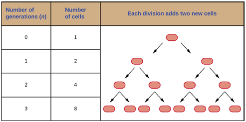
Generation Time: Recall that the most common mechanism of cell replication in bacteria is a process called binary fission, which is depicted in Figure 2.20. Also recall that when we are talking about microbial growth, we are talking about an increase in the number of cells in a population not about an increase in the size of the microbial cells themselves.

 

In eukaryotic organisms, the generation time is the time between the same points of the life cycle in two successive generations. For example, the typical generation time for the human population is 25 years. This definition is not practical for bacteria, which may reproduce rapidly or remain dormant for thousands of years. In prokaryotes (Bacteria and Archaea), the generation time is also called the doubling time and is defined as the time it takes for the population to double through one round of binary fission. Bacterial doubling times vary enormously. Whereas Escherichia coli can double in as little as 20 minutes under optimal growth conditions in the laboratory, bacteria of the same species may need several days to double in especially harsh environments. Most pathogens grow rapidly, like E. coli, but there are exceptions. For example, Mycobacterium tuberculosis, the causative agent of tuberculosis, has a generation time of between 15 and 20 hours. On the other hand, M. leprae, which causes leprosy, grows much more slowly, with a doubling time of 14 days.

 

Due to the population of the bacterial culture doubling each generation, bacterial grow exponentially, with each subsequent generation giving rise to twice as many daughter cells through the process of binary fission (Figure 5.16).  Due to this, bacteria can multiply to produce incredible numbers of cells within a very short period of time. For example, under ideal conditions, E. coli divides every 20mins, so over a single day a single cell could produce over a thousand, billion, billion cells, or approximately 3 cubic kilometers of cells.

 

Bacterial Growth Curves: Microorganisms grown in closed culture (also known as a batch culture), in which no nutrients are added and most waste is not removed, follow a reproducible growth pattern referred to as the growth curve. An example of a batch culture in nature is a pond in which a small number of cells grow in a closed environment. The culture density is defined as the number of cells per unit volume. In a closed environment, the culture density is also a measure of the number of cells in the population. Infections of the body do not always follow the growth curve, but correlations can exist depending upon the site and type of infection. When the number of live cells is plotted against time, distinct phases can be observed in the curve (Figure 5.17).

 

 

 

 

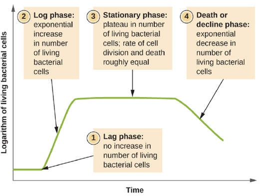
1. The Lag Phase: The beginning of the growth curve represents a small number of cells, referred to as an inoculum, that are added to a fresh culture medium, a nutritional broth that supports growth. The initial phase of the growth curve is called the lag phase, during which cells are gearing up for the next phase of growth. The number of cells does not change during the lag phase; however, cells grow larger and are metabolically active, synthesizing proteins needed to grow within the medium. If any cells were damaged or shocked during the transfer to the new medium, repair takes place during the lag phase. The duration of the lag phase is determined by many factors, including the species and genetic make-up of the cells, the composition of the medium, and the size of the original inoculum.

 

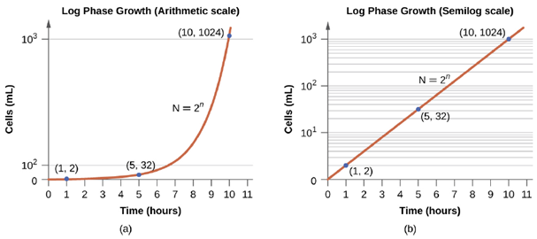
2. The Log Phase: In the logarithmic (log) growth phase, sometimes called exponential growth phase, the cells are actively dividing by binary fission and their number increases exponentially. For any given bacterial species, the generation time under specific growth conditions (nutrients, temperature, pH, and so forth) is genetically determined, and this generation time is called the intrinsic growth rate. During the log phase, the relationship between time and number of cells is not linear but exponential; however, the growth curve is often plotted on a semilogarithmic graph, as shown in Figure 5.18, which gives the appearance of a linear relationship.

 

 

Cells in the log phase show constant growth rate and uniform metabolic activity. For this reason, cells in the log phase are preferentially used for industrial applications and research work. The log phase is also the stage where bacteria are the most susceptible to the action of disinfectants and common antibiotics that affect protein, DNA, and cell-wall synthesis.

 

3. Stationary Phase: As the number of cells increases through the log phase, several factors contribute to a slowing of the growth rate. Waste products accumulate and nutrients are gradually used up. In addition, gradual depletion of oxygen begins to limit aerobic cell growth. This combination of unfavorable conditions slows and finally stalls population growth. The total number of live cells reaches a plateau referred to as the stationary phase (Figure 5.17). In this phase, the number of new cells created by cell division is now equivalent to the number of cells dying; thus, the total population of living cells is relatively stagnant. The culture density in a stationary culture is constant. The culture’s carrying capacity, or maximum culture density, depends on the types of microorganisms in the culture and the specific conditions of the culture; however, carrying capacity is constant for a given organism grown under the same conditions.

During the stationary phase, cells switch to a survival mode of metabolism. As growth slows, so too does the synthesis of peptidoglycans, proteins, and nucleic-acids; thus, stationary cultures are less susceptible to antibiotics that disrupt these processes. In bacteria capable of producing endospores, many cells undergo sporulation during the stationary phase. Secondary metabolites, including antibiotics, are synthesized in the stationary phase. In certain pathogenic bacteria, the stationary phase is also associated with the expression of virulence factors, products that contribute to a microbe’s ability to survive, reproduce, and cause disease in a host organism. For example, quorum sensing in Staphylococcus aureus initiates the production of enzymes that can break down human tissue and cellular debris, clearing the way for bacteria to spread to new tissue where nutrients are more plentiful.

 

4. The Death Phase: As a culture medium accumulates toxic waste and nutrients are exhausted, cells die in greater and greater numbers. Soon, the number of dying cells exceeds the number of dividing cells, leading to an exponential decrease in the number of cells (Figure 5.17). This is the aptly named death phase, sometimes called the decline phase. Many cells lyse and release nutrients into the medium, allowing surviving cells to maintain viability and form endospores.

 

Measurement of Bacterial Growth: Estimating the number of bacterial cells in a sample, known as a bacterial count, is a common task performed by microbiologists. The number of bacteria in a clinical sample serves as an indication of the extent of an infection. Quality control of drinking water, food, medication, and even cosmetics relies on estimates of bacterial counts to detect contamination and prevent the spread of disease. Two major approaches are used to measure cell number. The direct methods involve counting cells, whereas the indirect methods depend on the measurement of cell presence or activity without actually counting individual cells. Both direct and indirect methods have advantages and disadvantages for specific applications.

 

1. Direct Cell Count: Direct cell count refers to counting the cells in a liquid culture or colonies on a plate. It is a direct way of estimating how many organisms are present in a sample. Let’s look first at a simple and fast method that requires only a specialized slide and a compound microscope.

 

The simplest way to count bacteria is called the direct microscopic cell count, which involves transferring a known volume of a culture to a calibrated slide and counting the cells under a light microscope. The calibrated slide is called a Petroff-Hausser chamber (Figure 5.19) and is similar to a hemocytometer used to count red blood cells. The central area of the counting chamber is etched into squares of various sizes. A sample of the culture suspension is added to the chamber under a coverslip that is placed at a specific height from the surface of the grid. It is possible to estimate the concentration of cells in the original sample by counting individual cells in a number of squares and determining the volume of the sample observed. The area of the squares and the height at which the coverslip is positioned are specified for the chamber.

 

 

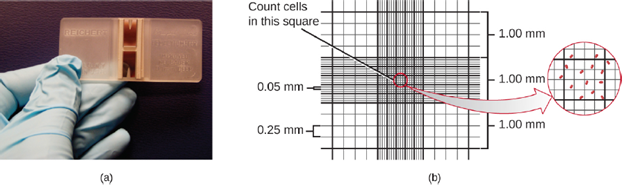
Cells in several small squares must be counted and the average taken to obtain a reliable measurement. The advantages of the chamber are that the method is easy to use, relatively fast, and inexpensive. On the downside, the counting chamber does not work well with dilute cultures because there may not be enough cells to count. Also, a counting chamber does not necessarily yield an accurate count of the number of live cells because it is not always possible to distinguish between live cells, dead cells, and debris of the same size under the microscope, or to count quickly moving cells.

 

2. Plate Count: The viable plate count, or simply plate count, is a count of viable or live cells. It is based on the principle that viable cells replicate and give rise to visible colonies when incubated under suitable conditions for the specimen. The results are usually expressed as colony-forming units per milliliter (CFU/mL) rather than cells per milliliter because more than one cell may have landed on the same spot to give rise to a single colony. Furthermore, samples of bacteria that grow in clusters or chains are difficult to disperse and a single colony may represent several cells. Some cells are described as viable but non-culturable and will not form colonies on solid media. For all these reasons, the viable plate count is considered a low estimate of the actual number of live cells. These limitations do not detract from the usefulness of the method, which provides estimates of live bacterial numbers.

 

Microbiologists typically count plates with 20–200 colonies. Samples with too few colonies (<20) do not give statistically reliable numbers, and overcrowded plates (>200 colonies) make it difficult to accurately count individual colonies. Also, counts in this range minimize occurrences of more than one bacterial cell forming a single colony. Thus, the calculated CFU is closer to the true number of live bacteria in the population. Most bacterial cultures are at concentrations in the millions or billions of CFUs/ml, so we must dilute our starting cultures before we put them onto plates. This is done through a process called serial dilution.

 

The goal of the serial dilution process is to obtain plates with CFUs in the range of 20–200, and the process usually involves several dilutions in multiples of 10 to simplify calculation. The number of serial dilutions is chosen according to a preliminary estimate of the culture density. Figure 5.20 illustrates the serial dilution method.

 

 

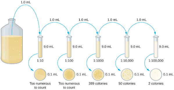
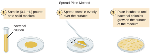
A fixed volume of the original culture, 1.0 mL, is added to and thoroughly mixed with the first dilution tube solution, which contains 9.0 mL of sterile broth. This step represents a dilution factor of 10, or 1:10, compared with the original culture. From this first dilution, the same volume, 1.0 mL, is withdrawn and mixed with a fresh tube of 9.0 mL of dilution solution. The dilution factor is now 1:100 compared with the original culture. This process continues until a series of dilutions is produced that will bracket the desired cell concentration for accurate counting. From each tube, a sample is plated on solid medium, usually by spread plating (Figure 5.21), and the plates are incubated until colonies appear. Two to three plates are usually prepared from each dilution and the numbers of colonies counted on each plate are averaged. In all cases, thorough mixing of samples with the dilution medium (to ensure the cell distribution in the tube is random) is paramount to obtaining reliable results.

 

 

The dilution factor is used to calculate the number of cells in the original cell culture. In our example, an average of 50 colonies was counted on the plates obtained from the 1:10,000 dilution. Because only 0.1 mL of suspension was pipetted on the plate, the multiplier required to reconstitute the original concentration is 10 × 10,000. The number of CFU per mL is equal to 50 × 10 × 10,000 = 5,000,000. The number of bacteria in the culture is estimated as 5 million cells/mL. The colony count obtained from the 1:1000 dilution was 389, well below the expected 500 for a 10-fold difference in dilutions. This highlights the issue of inaccuracy when colony counts are greater than 300 and more than one bacterial cell grows into a single colony. Direct plate counts are very accurate. Since we are counting colonies and colonies arise from living cells, dead cells are never counted in this method. One major disadvantage to using plate counts, is that they are time consuming, as serial dilutions must be prepared and cultures must be incubated, which might take several days to show colonies.

 

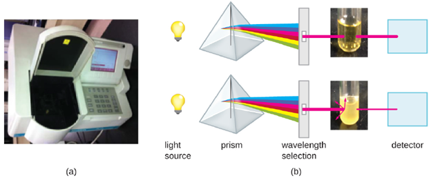
3. Indirect Methods: Besides direct methods of counting cells, other methods, based on an indirect detection of cell density, are commonly used to estimate and compare cell densities in a culture. The foremost approach is to measure the turbidity (cloudiness) of a sample of bacteria in a liquid suspension. The laboratory instrument used to measure turbidity is called a spectrophotometer (Figure 5.22). In a spectrophotometer, a light beam is transmitted through a bacterial suspension, the light passing through the suspension is measured by a detector, and the amount of light passing through the sample and reaching the detector is converted to either percent transmission or a logarithmic value called absorbance (optical density). As the numbers of bacteria in a suspension increase, the turbidity also increases and causes less light to reach the detector. The decrease in light passing through the sample and reaching the detector is associated with a decrease in percent transmission and increase in absorbance measured by the spectrophotometer.

 

Measuring turbidity is a fast method to estimate cell density as long as there are enough cells in a sample to produce turbidity. It is possible to correlate turbidity readings to the actual number of cells by performing a viable plate count of samples taken from cultures having a range of absorbance values. Using these values, a calibration curve is generated by plotting turbidity as a function of cell density. Once the calibration curve has been produced, it can be used to estimate cell counts for all samples obtained or cultured under similar conditions and with densities within the range of values used to construct the curve. One downside to turbidity measurements is that both live and dead cells are counted, so it is possible to get inaccurate results.