Packages
Plots
When including equations, it is often helpful to include plots and figures as a visual learning aid. The Tikz package provides a variety of tools for creating figures. The PGFplots package can be combined with Tikz to create simple to code yet elegant plots.
2D Plots
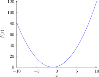
To create a plot, invoke the plot environment and then specify a few parameters including the axes and function to plot.
|
|
[latex] |
Code like this can seem overwhelming, but it becomes easier to read if you parse it one line at a time.
\begin{tikzpicture}starts the tikzpicture environment. Tikzpicture is an environment often used for drawing figures with geometric shapes or plots.\begin{axis}starts configuring the axes. The ‘[‘ at the end of the line indicates that we are going to enter some parameters for the axes.axis lines = left, means that the axes will be along the bottom and on the lefthand side.xlabel = $x$andylabel = {$f(x)$}specify that the x-axis should be labeled x and the y-axis should be labelled f(x). The brackets around $f(x)$ ensure that the whole group is made into the label. The ‘$’s means that the text will formatted like it is in math mode.- The ‘]’ ends the specifications for the axes.
\addplotadds a new plot to the figure.domain=-10:10, samples=30, color=blueconfigures the line on the figure, specifying it should range from x=-10 to x=10, that the plot should use 30 line segments, and that the color of the line should be blue. As you increase the number of line segments, the line becomes smoother. However, using more line segments uses more memory and results in the page loading slower.{x^2 + 2*x + 1};is the equation that will be plotted.\end{axis}and\end{tikzpicture}end the environments that we started earlier.
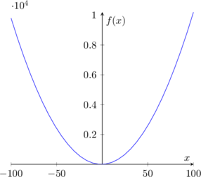
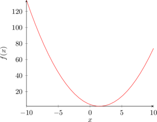
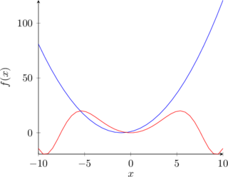
Understanding the code, we can modify the plot to show a wider range of values, modify the function, or plot an additional function on the same figure.
|
|
[latex] |
|
|
[latex] |
|
|
[latex] |
3D Plots
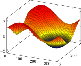
PGFPlots can also create 3D plots. The code for a 3D plot is similar to the 2D plot. Note that in this case we are setting the bounds for the axes in the parameters for addplot3 with the argument ‘domain=0:360’.
|
|
[latex] |
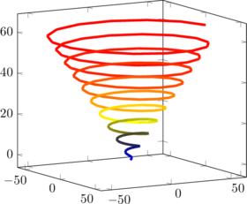
Here is another example of a 3D plot where we use all three dimensions to create a spiral.
|
|
[latex] |
- The two numbers given as parameters to the axes specify what angle you will see that plot at. The first argument specifies the rotation of the x-y plane and the second argument specifies the rotation in z.
- The
meshargument in addplot creates the color gradient. - The
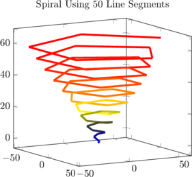
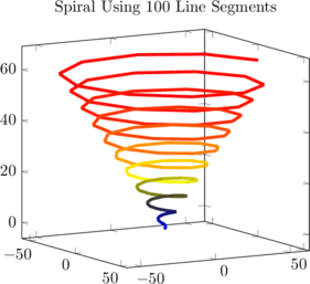
samples = 200argument says tells the plot how many line segments to generate. Note that in this case we had to use 150 samples in comparison to the 30 samples used for the other examples. The plot below shows what the spiral looks like with 50 and 100 samples.
- The function specifies the spiral with a function for each coordinate in terms of a single variable. This type of function is called a parametric function.
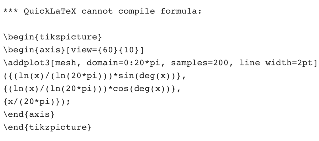
The y samples = 0 specifies that we are defining the line in terms of a single parameter. If you do not include this, Latex will generate an error. It is not obvious that you need this parameter, and the error doesn’t make it obvious what to change:
When doing something new with a package, such as creating a new type of plot, it is often easiest to learn from examples. The package documentation is often a good source of examples and will also help you figure out what arguments can be used. Here is the package documentation for PGFPlot. You can usually find the documentation of a package just by Googling the name of that package and documentation.

