Plot Solutions

These answers show one possible solution to each problem. Other ways of solving the problems are also correct.

1. The answers below show what portion of the code to change.
   1. \addplot [domain=-2:2, samples=100, color=blue]
   2. \begin{axis}[axis lines = left, xlabel = $x$, ylabel = $y$]
   3. \addplot [domain=-2:2, samples=100, color=green]
   4. \addplot [domain=-2:2, samples=100, color=blue]
{x^2 + 2*x + 1};

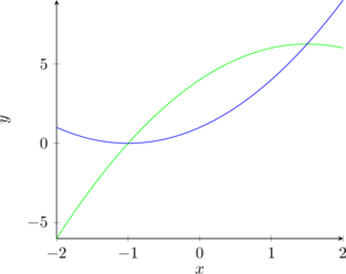
   [‌latex] \begin{tikzpicture} \begin{axis}[ axis lines = left, xlabel = $x$, ylabel = $y$] \addplot [ domain=-2:2, samples=100, color=green] {-x^2 + 3*x + 4}; \addplot [domain=-2:2, samples=100, color=blue] {x^2 + 2*x + 1}; \end{axis} \end{tikzpicture}[/latex]

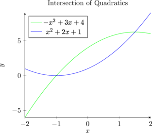
2. [‌latex] \begin{tikzpicture} \begin{axis}[axis lines = left, title=Intersection of Quadratics, xlabel = $x$, ylabel = $y$, legend pos= north west] \addplot [domain=-2:2, samples=100, color=green]{-x^2 + 3*x + 4}; \addplot [domain=-2:2, samples=100, color=blue]{x^2 + 2*x + 1}; \legend{$-x^2 + 3x + 4$,$x^2 + 2x + 1$} \end{axis} \end{tikzpicture}[/latex]

3. The first plot below uses a colorbar with point meta rel=axes wide, which maps the colorbar to the whole y axis. The second plot uses point meta rel=per plot which maps the colorbar to each function on the plot.
   

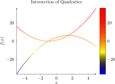
   	[‌latex] \begin{tikzpicture} \begin{axis}[axis lines=left, title=Intersection of Quadratics, xlabel=$x$, ylabel=$f(x)$, colorbar, point meta rel=axes wide, point meta=y] \addplot+[mesh, thick, mark=none] {-x^2 + 3*x + 4}; \addplot+[mesh, thick, mark=none] {x^2 + 2*x + 1}; \end{axis} \end{tikzpicture}[/latex]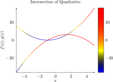
   	[‌latex] \begin{tikzpicture} \begin{axis}[axis lines=left, title=Intersection of Quadratics, xlabel=$x$, ylabel={$f(x), g(x)$}, colorbar, point meta rel=per plot, point meta=y] \addplot+[mesh, thick, mark=none] {-x^2 + 3*x + 4}; \addplot+[mesh, thick, mark=none] {x^2 + 2*x + 1}; \end{axis} \end{tikzpicture}[/latex]

4. The plot below shows the behavior of near 0. Note that if you increase the number of samples from 50 to 100, you will exceed the memory allotted for QuickLatex. In general, increasing the number of samples will reduce the responsiveness of your page. So, it is not always desirable to enter larger sample numbers.
   

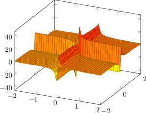
   [‌latex] \begin{tikzpicture} \begin{axis} \addplot3[surf, domain=-2:2, samples=40] {1/x + 1/y}; \end{axis} \end{tikzpicture} [/latex]

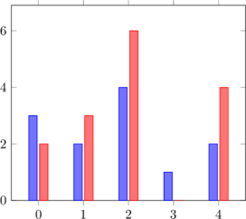
5. [‌latex] \begin{tikzpicture} \begin{axis}[ybar, enlarge y limits={0.15,upper}, enlarge x limits=0.15] \addplot plot coordinates {(0,3) (1,2) (2,4) (3,1) (4,2)}; \addplot plot coordinates {(0,2) (1,3) (2,6) (3,0) (4,4)}; \end{axis} \end{tikzpicture} [/latex]