7 Chapter 7 Redundancy, Functional Dependencies, Closure, and Normalization
Fred Strickland
Original Chapter 10 Author: Adrienne Watt
Original Chapter 11 Author: Adrienne Watt
Original Chapter 12 Author: Adrienne Watt
Rewrite: Fred Strickland
Learning Outcomes
Introduction to Chapter 7
Chapter 6 addressed the mechanisms for preventing bad or duplicate data from being entered into a database. We looked at integrity rules, constraints, and cardinality for ensuring the high quality of the data. From the “seat of the pants,” we figured out what tables we might need. What if you are starting with no suggestions and with no guidance? If you have extensive experience with spreadsheets, you might be tempted to create one huge database table. There are issues with this approach. There is a reasonable approach for avoiding these issues.
The Third Edition Style Guide
This is the style guide that this book will follow for this chapter and for the other chapters.
|
Naming Convention:
Using the IE’s Notation with Crow’s Foot Notation. |
Figure 7.1 The database style guide. Adapted from https://vertabelo.com/blog/database-schema-naming-conventions/
The Redundancy Issue
Redundancy is when data appears in some fashion two more times in a table. This is undesirable, because it causes problems.
|
Third edition |
||||||||||||||||||||||||||||||||||||||||||||||||||||||
|
||||||||||||||||||||||||||||||||||||||||||||||||||||||
|
Second Edition |
||||||||||||||||||||||||||||||||||||||||||||||||||||||
|
|
||||||||||||||||||||||||||||||||||||||||||||||||||||||
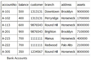
Figure 7.2 Example of a table containing redundant data. The bottom image is a reproduction of Figure 10.1 from the second edition (A. Watt).
In Figure 7.2, Customer 1313131 appears twice, because of two accounts (A-101 and A102). This is true for Customer 976543 and for 1111111. What could go wrong?
Insertion Anomaly
An insertion anomaly occurs when you are inserting inconsistent information into a table. When we insert a new record, such as account number A-306 in Figure 7.3, we need to check that the branch data is consistent with existing rows.
|
Third edition |
||||||||||||||||||||||||||||||||||||||||||||||||||||||||||||
|
||||||||||||||||||||||||||||||||||||||||||||||||||||||||||||
|
Second Edition |
||||||||||||||||||||||||||||||||||||||||||||||||||||||||||||
|
|
||||||||||||||||||||||||||||||||||||||||||||||||||||||||||||
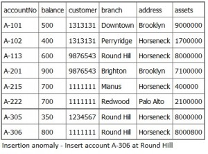
Figure 7.3 Example of an insertion anomaly. The bottom image is a reproduction of Figure 10.2 from the second edition (A. Watt).
The issue is that the asset boxes for A-113 and for A-305 do not agree with the figure for A-306. To keep the data consisted, we would need to revise the figures for these other two accounts.
Update Anomaly
The last paragraph was a hint to this issue. An update anomaly occurs when you are updating data and similar rows need to be found and updated. Figure 7.4 shows this situation for the Round Hill branch.
|
Third edition |
||||||||||||||||||||||||||||||||||||||||||||||||||||||
|
||||||||||||||||||||||||||||||||||||||||||||||||||||||
|
Second Edition |
||||||||||||||||||||||||||||||||||||||||||||||||||||||
|
|
||||||||||||||||||||||||||||||||||||||||||||||||||||||
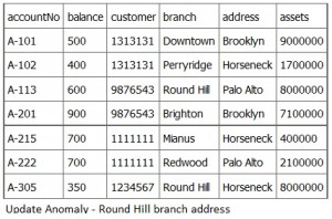
Figure 7.4 Example of an update anomaly. The bottom image is a reproduction of Figure 10.3 from the second edition (A. Watt).
The issue here is that the Round Hill address has changed from Horseneck to Palo Alto. A-113 was updated, but A-305 data was not updated.
Deletion Anomaly
A deletion anomaly occurs when you are deleting data and the record contains data that might be important to retain. Figure 7.5 shows that A-101 is the last account at the Downtown branch. If we delete this record, then we lose access to the Downtown branch address and to the asset figure.
|
Third edition |
||||||||||||||||||||||||||||||||||||||||||||||||||||||
|
||||||||||||||||||||||||||||||||||||||||||||||||||||||
|
Second Edition |
||||||||||||||||||||||||||||||||||||||||||||||||||||||
|
|
||||||||||||||||||||||||||||||||||||||||||||||||||||||
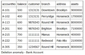
Figure 7.5 Example of an update anomaly. The bottom image is a reproduction of Figure 10.4 from the second edition (A. Watt).
Fortunately, Customer 1313131 has an account at the Perryridge branch. Otherwise, we would have lost access to the existence of Customer 1313131.
Functional Dependency
How do we break this large table into smaller tables? We could break the large table into two tables such as:
- Customers
- AccountNumber
- Balance
- CustomerID
- Branches
- Branch
- Address
- Asset
What about the customer’s address and contact data? What about the branch manager data, the employees assigned, and the contact data? Should these items be added to these two tables or stored in a new table?
Functional dependency (FD) is a relationship between attributes such as between the PK and the non-key attributes. Something determines the other attributes. An FD is a database constraint that determines the relationship of one attribute to another attribute. FDs help to maintain the quality of data in a database.
FD are expressed as an “equation.” The variable (the determinant) on the left side of the arrow determines the attributes (the dependent) on the right side.
- Second Edition: X —-> Y and A —-> B
- Third Edition: A–> B1 and A –> B
Here are some word examples:
- In the Employees table: ID would determine the FirstName and the LastName.
- In the Students table: ID would determine the FirstName, the LastName, and the ClassRank.
- In the Branches table: ID would determine the Name, the Address, and the Assets.
- In a table collecting data: SIN or SSN would determine the Name, the Address, and the Birthdate.
- In a table collecting data: ISBN would determine the Title and other pieces of data.
Some FDs are easy to figure out. Other FDs are not. Consider the following table:
|
A |
B |
C |
D |
E |
|
a1 |
b1 |
c1 |
d1 |
e1 |
|
a2 |
b1 |
c2 |
d2 |
e1 |
|
a3 |
b2 |
c1 |
d1 |
e1 |
|
a4 |
b2 |
c2 |
d2 |
e1 |
|
a5 |
b3 |
c3 |
d1 |
|
Table 7.1 Functional dependency table example. This is a corrected reproduction of Figure 10.4 from the second edition (A. Watt).
Which columns contain unique values? The answer is column A. So column A can be used to determine the values of the other columns. We can write this as:
|
Single Letters |
Double Letters |
Triple Letters |
Quadruple Letters |
|
|
|
|
Table 7.2 Functional dependencies from the viewpoint of A.
Other columns may be used to determine other columns. In this example, the values in column E are the same. So any column could be used to determine the value in column E.
The fact that column A could be used to determine the values of the other columns may be summarized as A –> BCDE. We can conclude that A must be a PK.
Recall from Chapter 5 that a composite key uses more than one attribute to locate a record. By inspection, we see that the pairing of B and C is unique and the pairing of B and D is unique. The PK of A may be used in combination with other values. These pairings are shown in the next table:
|
B |
C |
Functional Dependencies |
|
b1 |
c1 |
BC –> A BC –> DE BC –> ADE |
|
b1 |
c2 |
|
|
b2 |
c1 |
|
|
b2 |
c2 |
|
|
b3 |
c3 |
|
|
|
|
|
|
B |
D |
Functional Dependencies |
|
b1 |
d1 |
BD –> A BD –> CE BD –> ACE |
|
b1 |
d2 |
|
|
b2 |
d1 |
|
|
b2 |
d2 |
|
|
b3 |
d1 |
|
|
|
|
|
|
A |
B |
Functional Dependencies |
|
a1 |
b1 |
AB –> C AB –> D AB –> E AB –> CD AB –> CE AB –> DE |
|
a2 |
b1 |
|
|
a3 |
b2 |
|
|
a4 |
b2 |
|
|
a5 |
b3 |
|
Table 7.3 Functional dependencies from the viewpoint of a composite key.
Some values are uniquely linked to other values. A value of C always points to the same value of D:
|
C |
D |
Functional Dependencies |
|
c1 |
d1 |
C –> D |
|
c2 |
d2 |
|
|
c1 |
d1 |
|
|
c2 |
d2 |
|
|
c3 |
d1 |
|
Table 7.4 Localized Functional dependencies.
Since E is the same for each line, then we have other determinants:
|
Table 7.5 Additional determinants for accessing dependent E.
The determinant and dependent relationship tends to be one way. The following table demonstrates this point:
|
Proposed Determinant and Dependent Relationship |
Reason for the Failure |
|
E –> anything |
Since the values of E are the same, there is no way to determine a unique value in another column. |
|
D –> C |
Value d1 points to value c1 and to value c3. |
|
D –> B |
Value d1 points to value b1 and to value b2 |
|
D –> A |
Value d1 points to value a1 and to value a3. |
|
C –> B |
Value c1 points to value b1 and to value b2. |
|
C –> A |
Value c1 points to value a1 and to value a3. |
|
B –> A |
Value b1 points to value a1 and to value a2. |
Table 7.6 Invalid determinant-dependent relationships.
Using the new understanding of FD and the FD equation or shorthand, we can express the five examples as:
|
In the Employees table: ID would determine the FirstName and the LastName. |
ID –> FirstName, LastName |
|
In the Students table: ID would determine the FirstName, the LastName, and ClassRank. |
ID –> FirstName, LastName, ClassRank |
|
In the Branches table: ID would determine the Name, the Address, and the Assets. |
ID –> Name, Address, Assets |
|
In a table collecting data: SIN or SSN would determine the FirstName, the LastName, the Address, and the Birthdate. |
SIN –> FirstName, LastName, Address, Birthdate SSN –> FirstName, LastName, Address, Birthdate |
|
In a table collecting data: ISBN would determine the Title and other pieces of data |
ISBN –> Title |
Figure 7.6 Examples of expressing the previous example database tables in the FD shorthand.
There are several types of functional dependency relationships.
Trivial Functional Dependency
The dependent is a subset of the determinant. For example, a database table might have an ID column and an employee name column. If the functional dependency was written as {ID, EmployeeName} –> ID, then this is a trivial functional dependency. This is true, because the dependent ID appears in the determinant list.
DatabaseTown noted that this could be done with a composite key as (Order ID, Customer ID) –> (Customer ID).
Non-Trivial Functional Dependency
The dependent is not a subset of the determinant. The examples in Figure 7.6 are non-trivial functional dependency, because the elements in the right set are not a subset of the left side.
Multivalued Functional Dependency
The Geeks for Geeks writer (“What is Functional Dependency in DBMS?”) explained this as two or more values in a cell. Figure 7.7 shows a simple example of this viewpoint for a Students table:
|
ID |
StudentName |
Course |
|
101 |
Ali |
{Math, English} |
|
102 |
Bob |
{History, English} |
|
103 |
Cavin |
{Physics, Hindi} |
|
ID –> Courses |
||
|
101 –> {Math, English} 102 –> {History, English} 103 –> {Physics, Hindi} |
||
Figure 7.7 Geeks for Geeks example of a multivalued functional dependency. (The ID column was changed to follow the style guide.)
Fiona Brown and other writers have a different understanding. Fiona Brown wrote:
Multivalued dependency occurs in the situation where there are multiple independent multivalued attributes in a single table. A multivalued dependency is a complete constraint between two sets of attributes in a relation. It requires that certain tuples be present in a relation.
Fiona Brown used a Cars table to explain this functional dependency:
|
CarModel |
ManufactureYear |
Color |
|
H001 |
2017 |
Metallic |
|
H001 |
2017 |
Green |
|
H005 |
2018 |
Metallic |
|
H005 |
2018 |
Blue |
|
H010 |
2015 |
Metallic |
|
H033 |
2012 |
Gray |
|
The manufacture year and the color values are independent of each other but dependent on the car model. In this example, these two columns are said to be multivalue dependent on the car model. |
||
|
CarModel –> ManufactureYear CarModel –> Color |
||
Figure 7.8 The Fiona Brown example of a multivalued functional dependency. (The first two columns were changed to follow the style guide.)
Another Geeks for Geeks writer had a different example with a different explanation:
|
RollNumber |
Name |
Age |
|
42 |
abc |
17 |
|
43 |
pqr |
18 |
|
44 |
xyz |
18 |
|
45 |
abc |
19 |
|
[The] entities of the dependent set are not dependent on each other. i.e. If a → {b, c} and there exists no functional dependency between b and c, then it is called a multivalued functional dependency. Here, roll_no → {name, age} is a multivalued functional dependency, since the dependents name & age are not dependent on each other(i.e. name → age or age → name doesn’t exist !) |
||
|
RollNumber –> {Name, Age} |
||
Figure 7.9 A different Geeks for Geeks example of a multivalued functional dependency. (The column names were changed to follow the style guide.)
Transitive Functional Dependency
One column determines a column and that column determines another column. Using the table collecting data example from Figure 7.6, this could be illustrated as follows:
|
SINorSSN |
FirstName |
LastName |
Address |
Birthdate |
|
123 |
Mary |
Smith |
Toronto |
September 9 |
|
234 |
James |
Johnson |
Orlando |
September 19 |
|
345 |
Patricia |
Williams |
Vancouver |
September 12 |
|
456 |
John |
Brown |
Las Vegas |
September 17 |
Figure 7.10 An example of a transitive functional dependency.
With the SIN or SSN, we know the person’s name. If we know the person’s name, then we can learn what is the birthday. So according to this FD, we can learn the birthday with the SIN or SSN. Here are the shorthand expressions:
- {SINorSSN} –> {FirstName, LastName}
- {FirstName, LastName} –> Birthdate
- {SINorSSN} –> Birthdate
In more formal way, this could be expressed as:
If A –> B and B –> C, then A –> C
Full Functional Dependency and Partial Functional Dependency
Some sources will include two more FDs. These appear to be more of a description of how the determinant and the dependent are related.
A full FD is when the determinant determines all the columns in a table.
- {OrderID} –> {OrderID, CustomerID, ProductID, Quantity}
A partial FD is when a determinant piece determines some of the columns in a table.
- {OrderID, CustomerID} –> {ProductID, Quantity}
The Advantages and the Disadvantages of Working with Functional Dependencies
Advantages of Working with Functional Dependency
- We are able to identify the primary key and the candidate keys.
- We can define the tables and the needed attributes. This helps in query optimization and thus improves performance.
- We can ensure that the data is consist by removing redundancies and inconsistencies.
- We can ensure that the data is accurate, complete, and current.
Disadvantages of Working with Functional Dependency
- We may spend much time in the process of identifying the FDs in a large database that has many tables with many relationships.
- Some use a dependency diagram. This has the appearance of a row of boxes with arrows coming out of the top and bottom. The second edition provided an example as Figure 11.6 and as Figure 12.1. The accompanying text listed the dependencies, but did not provide instructions on how to create a dependency diagram. Some older database textbooks do address this topic. In the recently dated web pages, none used a dependency diagram. It appears that dependency diagrams have fallen out of favor7. So this edition will not address this topic.
- We may find the FDs to be overly restrictive and may result in slow query performance.
- We may find that the FDs do not take into account the semantic meanings of our data and thus may not always reflect the true relationships between our data elements.
Functional Dependency Set and Attribute Closure
We will use the following Students table for this topic:
|
ID |
LastName |
Phone |
State |
Country |
Age |
|
123 |
Smith |
416-555-0000 |
ON |
Canada |
18 |
|
234 |
Johnson |
407-555-0000 |
FL |
United States |
19 |
|
345 |
Williams |
236-555-0000 |
BC |
Canada |
21 |
|
456 |
Brown |
702-555-0000 |
NV |
United States |
22 |
Table 7.6 Students table (Roughly based on https://www.geeksforgeeks.org/functional-dependency-and-attribute-closure/)
We know that ID –> LastName and that ID –> Phone are valid. LastName –> State is not valid. Why? There could be another Smith elsewhere in this table that lives in the same state or province.
FDs in a relation are dependent upon the domain of the relation. By inspection, we know the following are valid:
|
ID –> LastName |
State –> Country |
|
ID –> Phone |
|
|
ID –> State |
|
|
ID –> Country |
|
|
ID –> Age |
|
Figure 7.11 Valid functional dependencies for the Students table.
A functional dependent set (FD set) is the set of all FDs present in the relation. The following is the FD set for the Students table:
{ID –> LastName, ID –> Phone, ID –> State, ID –> Country, ID –> Age, State –> Country}
Attribute Closure
Attribute closure of an attribute set is defined as the set of attributes that can be functionally determined from it.
The steps for finding the attribute closure of an attribute set are:
- Add the elements of the attribute set to the result set.
- Recursively add the elements to the result set that can be functionally determined from the elements currently in the result set.
The custom is to mark the result set with a trailing plus (+) symbol and an equal (=) symbol pointing to the result set. The following shows the ID result set and the result set:
- (ID)+ = {ID, LastName, Phone, State, Country, Age}
- (State)+ = {State, Country}
Attribute Closure Advantages and Disadvantages
Attribute closure has the following advantages:
- Attribute closures help to identify all possible attributes that can be derived from a set of given attributes.
- Attribute closures facilitate database design by identifying relationships between attributes and tables that can help to optimize query performance.
- Attribute closures ensure data consistency by identifying all possible combinations of attributes that can exist in the database.
Attribute closure has the following disadvantages:
- The process of calculating attribute closures can be computationally expensive, especially for large databases.
- Attribute closures can become too complex to manage, especially as the number of attributes and tables in a database grows.
- Attribute closures do not take into account the semantic meaning of data and may not always accurately reflect the relationships between data elements.
Using Attribute Closure for Finding Candidate Keys and Super Keys
An attribute closure set that contains all possible attributes of relations is the super key. A candidate key is subset of the super key. The following will demonstrate this point:
- (ID, LastName)+ = {ID, LastName, Phone, State, Country, Age}
- (ID)+ = {ID, LastName, Phone, State, Country, Age}
The (ID, LastName)+ is the super key, but not a candidate key, because its subset (ID)+ is equal to all attributes of the relation. So ID would be a candidate key and a possible PK.
An Algorithm for Determining the Closure Set for a Functional Determinate
In an abstract conversation, the participants may use formal notation that looks like the following:
Given R (….)
FDs = {….}
Find (…)+
This is a formal way of finding a candidate key or a super key. The following shows the steps for solving a formal closure problem:
- Read the problem:
- Given the relation R (A, B, C, D, E) and the following FDs:
- {A –> B, B –> C, C –> D, D –> E)
- What is {A}+?
- Given the relation R (A, B, C, D, E) and the following FDs:
- A will be in the result set. So we add it to the result set: {A}+ = {A}
- What columns can be determined for a given A? We found A –> B from the FD list. So we add B to the result set: {A}+ = {A, B}
- Since we have A and B in the result set, we can look for any FD that has B as the determinant. We found B –> C from the FD list. So we add C to the result set: {A}+ = {A, B, C}
- We will repeat what we did for step 4 for the new letter. And we will continue repeating until we are finished:
- With C, we found C –> D from the FD list. So we add D to the result set: {A}+ = {A, B, C, D|
- With D, we found D –> E from the FD list. So we add E to the result set: {A}+ = {A, B, C, D, E}
- The last letter has been used. So the result set is {A}+ = {A, B, C, D, E}
The previous example was easy to understand and to solve. When a composite determinate is used, then the effort is more challenging. Here is such an example:
- Read the problem:
- Given the relation R (A, B, C, D, E, F). and the following FDs:
- {AB –> C, BC –> AD, D –> E, CF –> B)
- What is {A, B}+?
- A and B will be in the result set based on the FD list. So we add these two to the result set: {A, B}+ = {A, B}
- What columns can be determined for a given A and B combination? We found AB C from the FD list. So we add C to the result set: {A, B}+ = {A, B, C}
- What single letter or combinations from the result set could help us to find another letter? We found BC AD from the FD list. So we add D. A is already present in the result set. Now we have: {A, B}+ = {A, B, C, D}
- What single letter or combinations from the result set could help us to find another letter? We found D E from the FD list. So we add E to the result set: {A, B,}+ = {A, B, C, D, E}
- The remaining column is F. We cannot add it to the result set, because it was not in the determinant set and no letter pointed to it.
- So the result set is {A, B}+ = {A, B, C, D, E}
Armstrong’s Axioms in Functional Dependency (in DBMS)
William W. Armstrong defined some tests or inference rules about how to derive other FDs. There are three Armstrong’s Axioms and six secondary rules. Some sources listed six inference rules. We will follow the approach of defining three axioms followed by six secondary rules:
|
Axiom of Reflexivity: |
If A is a set of attributes and B is a subset of A, then A holds B. If B ⊆ A then A → B. This is the trivial property. |
|
Axiom of Augmentation: |
If A → B holds and Y is the attribute set, then AY → BY also holds. That is, adding attributes to dependencies, does not change the basic dependencies. If A → B, then AC → BC for any C. |
|
Axiom of Transitivity: |
If A → B holds and B → C holds, then A → C also holds. A → B is also called functionally that determines B. If X → Y and Y → Z, then X → Z. |
|
Secondary Rule of Union: |
If A→B holds and A→C holds, then A→BC holds. If X→Y and X→Z then X→YZ. |
|
Secondary Rule of Composition: |
If A→B and X→Y hold, then AX→BY holds. |
|
Secondary Rule of Decomposition: |
If A→BC holds then A→B and A→C hold. If X→YZ then X→Y and X→Z. |
|
Secondary Rule of Pseudo Transitivity: |
If A→B holds and BC→D holds, then AC→D holds. If X→Y and YZ→W then XZ→W. |
|
Secondary Rule of Self Determination: |
It is similar to the Axiom of Reflexivity, i.e. A→A for any A. |
|
Secondary Rule of Extensivity: |
Extensivity is a case of augmentation. If AC→A, and A→B, then AC→B. Similarly, AC→ABC and ABC→BC. This leads to AC→BC. |
Figure 7.12 Armstrong’s three Axioms and six secondary rules.
Now to apply these axioms and rules to the example problem:
|
Read the problem: Given the relation R (A, B, C, D, E, F). and the following FDs: {AB –> C, BC –> AD, D –> E, CF –> B) What is {A, B}+? |
|
|
A and B will be in the result set. So we add it to the result set: {A, B}+ = {A, B} |
This is understood. The rule of Self Determination. |
|
What columns can be determined for a given A and B combination? We found AB C. So we add C to the result set: {A, B}+ = {A, B, C} |
It came from the FD list. |
|
What single letter or combinations from the result set could help us to find another letter? We found BC –> AD. So we add D. A is already present in the result set. Now we have: {A, B}+ = {A, B, C, D} |
It came from the FD list. |
|
What single letter or combinations from the result set could help us to find another letter? We found D –> E. So we add E to the result set: {A, B,}+ = {A, B, C, D, E} |
It came from the FD list. |
|
The remaining column is F. We cannot add it to the result set, because it was not in the determinant set and no letter pointed to it. |
|
|
So the result set is {A, B}+ = {A, B, C, D, E} |
|
Figure 7.13 Armstrong’s three Axioms and six secondary rules applied to an example problem.
Armstrong’s Axioms and Rules work better when you are trying to calculate some members. The following example is adapted from the TutorialRide.com web page:
|
Relation R: |
(P, Q, R, S, T, U) |
|||||
|
FDs: |
P –> Q |
P –> R |
QR –> S |
|||
|
Q –> T |
QR –> U |
PR –> U |
||||
|
Calculate these members: |
P –> T |
PR –> S |
QR –> SU |
PR –> SU |
||
|
The Steps |
||||||
|
P –> T From the FD list, we have P –> Q and Q –> T. Using the Transitivity Axiom: If {A → B} and {B → C}, then {A → C} We can obtain P T. |
||||||
|
PR –> S From the FD list, we have P –> Q and QR –> S. Using the Pseudo Transitivity Rule: If {A → B} and {BC → D}, then {AC → D} We can obtain PR –> S. |
||||||
|
QR –> SU From the FD list, we have QR –> S and QR –> U. Using the Union Rule: If {A → B} and {A → C}, then {A → BC} We can obtain QR –> SU. |
||||||
|
PR –> SU From the FD list, we have P –> Q, QR –> S, and PR –> U Using the Pseudo Transitivity Rule: If {A → B} and {BC → D}, then {AC → D} We can obtain PR –> S. Using the Pseudo Transitivity Rule: If {A → B} and {BC → D}, then {AC → D} We use PR –> S with PR –> U and obtain PR –> SU. |
||||||
Figure 7.14 Armstrong’s three Axioms and six secondary rules applied to another example problem.
Advantages and Disadvantages of Using Armstrong’s Axioms
The advantages are:
- These provide a systematic and efficient method for inferring additional functional dependencies from a given set of functional dependencies, which can help to optimize database design.
- These can be used to identify redundant functional dependencies, which can help to eliminate unnecessary data and improve database performance.
- These can be used to verify whether a set of functional dependencies is a minimal cover, which is a set of dependencies that cannot be further reduced without losing information.
Some writers will mention the words “sound” and “complete” when discussing the advantages of using Armstrong’s Axioms. They are stating that:
- Sound means that for a given set of FDs that are specified for a relation schema , a person should be able infer any dependency from the FDs by using the primary rules of Armstrong’s Axioms and that these will hold in every relation state of the relational schema R that satisfies the dependencies in the FDs.
- Complete means that for when using the primary rules of the Armstrong’s Axioms repeatedly for inferring other dependencies that continue until we reach a stopping point, we will have a complete set of dependencies.
Disadvantages are:
- The process of using Armstrong’s axioms to infer additional functional dependencies can be computationally expensive, especially for large databases with many tables and relationships.
- The axioms do not take into account the semantic meaning of data and may not always accurately reflect the relationships between data elements.
- The axioms can result in a large number of inferred functional dependencies that can be difficult to manage and maintain over time.
We could add a fourth disadvantage. It is hard to grasp and to apply!
Normalization
Functional dependency and the supporting tools should make it easier to create and maintain the database. The given reasons are to:
- Ensure the integrity of the data.
- Provide insights when a database needs to be changed.
- Support normalization.
The idea is that database designers can use the identified dependencies in order to split large tables into smaller and thus more manageable tables. The same goal can be achieved by following the normalization rules.
Normalization is a step-by-step process for minimizing redundancy in a database. There are six normal forms. Taking a relational database to the first three would solve most issues.
Normalization:
- Makes the database more efficient.
- Prevents the same data from being stored in more than one place. The redundancy issue.
- Prevents updates being made to some data rows but not to other data. The update anomaly issue.
- Prevents data pieces from being deleted when the data should be retained. The delete anomaly issue.
- Ensures the data is accurate.
- Reduces the storage space that a database requires.
- Ensures that queries run as fast as possible.
- Avoids having very large relations.
We will be using the following “spreadsheet” like database table:
|
Student Name |
Fees Paid |
Date of Birth |
Address |
Phone |
Subject 1 |
Subject 2 |
Subject 3 |
Subject 4 |
Teacher Name11 |
Teacher Address |
Course Name |
|
Mary Smith |
18-Jul-00 |
09-Sep 91 |
3 Main Street, Toronto ON |
416-555-0000 416-555-9999 |
Economics 1 (Business) |
Biology 1 (Science) |
|
|
Suki Badh |
N4335H |
Economics |
|
James Johnson |
14-May-01 |
19-Sep-92 |
16 Leeds Road, Orlando FL |
407-555-0000 407-555-9999 |
Biology 1 (Science) |
Business Intro (Business) |
Programming 2 (IT) |
|
Nelson Eng |
N4335J |
Computer Studies & Information Systems |
|
Patricia Williams |
03-Feb-01 |
12-Sep-91 |
21 Arrow Street, Vancouver BC |
236-555-0000 236-555-9999 |
Biology 2 (Science) |
|
|
|
Jennifer Barker |
A3083 |
Biology |
|
John Brown |
29-Apr-02 |
17-Sep-92 |
14 Milk Lane, Las Vegas NV |
702-555-0000 702-555-9999 |
|
|
|
|
Jessie Clasen |
S3616 |
Biology |
Figure 7.15 A “spreadsheet” like database table.
This is a fine spreadsheet. We have the full name of a student. We know when they paid their fees. We know where they live. We see two contact phone numbers for each student. We can see some courses. We see information about the teachers.
But is this a useful spreadsheet? The columns for subjects contain many empty cells. We cannot tell if the instructor data is about a course or about an academic advisor area. We do not know when a course is being offered or if a student is repeating a course. We cannot tell anything about the schedule for a student. We cannot tell what courses an instructor is teaching.
First Normal Form (1NF)
First Normal Form (1NF) requires that each cell row is unique.
Ben who wrote “Database Normalization: A Step-By-Step-Guide With Examples” approached from a viewpoint that is different from other experts. To go from a “spreadsheet” database table to a First Normal Form (1NF) database table, he asks two questions:
- Does the combination of all columns make a unique row every single time?
- What field can be used to uniquely identify the row?
From looking at the data, the answer is “Yes” for the first question. However, a spreadsheet could have repeated lines. A database without a defined PK could have duplicated rows. So Ben answered the first question as “No.”
For the second question, we need to inspect each field. Could we use the student’s name as it is stored? The student’s name could be shared by another student. Address might work, but suppose a sibling joins an older sibling at the same address. That violates the idea of using a unique field. It may be tempting to use the student’s name plus another field, but that falls apart if another student with the same name comes into the same building.
The only solution is to create a new field with unique entries. While Ben’s approach is interesting and useful for 1NF, his discussion for 2NF is very long. You may read the rest of Ben’s approach by looking in the reference list. For the rest of this chapter, we will follow the more common approach to normalization.
The more common approach defines 1NF as a database table where each cell contains only one value. In the spreadsheet like database table, the phone column violates this requirement.
Here is the revision:
|
Student Name |
Fees Paid |
Date of Birth |
Address |
Phone |
Subject 1 |
Subject 2 |
Subject 3 |
Subject 4 |
Teacher Name12 |
Teacher Address |
Course Name |
|
Mary Smith |
18-Jul-00 |
09-Sep 91 |
3 Main Street, Toronto ON |
416-555-0000
|
Economics 1 (Business) |
Biology 1 (Science) |
|
|
Suki Badh |
N4335H |
Economics |
|
Mary Smith |
18-Jul-00 |
09-Sep 91 |
3 Main Street, Toronto ON |
416-555-9999 |
Economics 1 (Business) |
Biology 1 (Science) |
|
|
Suki Badh |
N4335H |
Economics |
|
James Johnson |
14-May-01 |
19-Sep-92 |
16 Leeds Road, Orlando FL |
407-555-0000
|
Biology 1 (Science) |
Business Intro (Business) |
Programming 2 (IT) |
|
Nelson Eng |
N4335J |
Computer Studies & Information Systems |
|
James Johnson |
14-May-01 |
19-Sep-92 |
16 Leeds Road, Orlando FL |
407-555-9999 |
Biology 1 (Science) |
Business Intro (Business) |
Programming 2 (IT) |
|
Nelson Eng |
N4335J |
Computer Studies & Information Systems |
|
Patricia Williams |
03-Feb-01 |
12-Sep-91 |
21 Arrow Street, Vancouver BC |
236-555-0000
|
Biology 2 (Science) |
|
|
|
Jennifer Barker |
A3083 |
Biology |
|
Patricia Williams |
03-Feb-01 |
12-Sep-91 |
21 Arrow Street, Vancouver BC |
236-555-9999 |
Biology 2 (Science) |
|
|
|
Jennifer Barker |
A3083 |
Biology |
|
John Brown |
29-Apr-02 |
17-Sep-92 |
14 Milk Lane, Las Vegas NV |
702-555-0000 |
|
|
|
|
Jessie Clasen |
S3616 |
Biology |
|
John Brown |
29-Apr-02 |
17-Sep-92 |
14 Milk Lane, Las Vegas NV |
702-555-9999 |
|
|
|
|
Jessie Clasen |
S3616 |
Biology |
Figure 7.16 The revised “spreadsheet” like database table.
This is an improvement, but there are still some issues that need to be addressed.
Second Normal Form (2NF)
Second Normal Form (2NF) requires that a database table is in 1NF and that each non-key attribute must be functionally dependent on the primary key.
To go from an improved “spreadsheet” database table to a Second Normal Form (2NF) database table, we need to ask one question:
- Does this column depend upon the PK?
The section on FDs provided the formal way of answering this question. Informally, we can determine this by asking a question about dependency upon the PK.
|
Student Name |
Yes, this is dependent on the PK. A different ID would mean a different student name. |
|
Fees Paid |
Yes, this is dependent on the PK. Each fees paid value is for a single student. |
|
Date of Birth |
Yes, it is specific to that student. |
|
Address |
Yes, it’s specific to that student. |
|
Subject 1 |
No, this column is not dependent on the student. More than one student could be enrolled in one subject. |
|
Subject 2 |
No. Same as for Subject 1. More than one subject is allowed. |
|
Subject 3 |
No. Same rule as subject 2. |
|
Subject 4 |
No. Same rule as subject 2 |
|
Teacher Name |
No. The teacher’s name is not dependent on the student. |
|
Teacher Address |
No. The teacher’s address is not dependent on the student. |
|
Course Name |
No. The course name is not dependent on the student. We still have the question about what this is really about. |
Figure 7.17 The specific questions for each column in the Students database table.
We can remove the “No” responses. Now our Students database table will have the following appearance:
|
StudentName |
FeesPaid |
DateOfBirth |
Address |
Phone |
|
Mary Smith |
18-Jul-00 |
09-Sep 91 |
3 Main Street, Toronto ON |
416-555-0000 |
|
Mary Smith |
18-Jul-00 |
09-Sep 91 |
3 Main Street, Toronto ON |
416-555-9999 |
|
James Johnson |
14-May-01 |
19-Sep-92 |
16 Leeds Road, Orlando FL |
407-555-0000 |
|
James Johnson |
14-May-01 |
19-Sep-92 |
16 Leeds Road, Orlando FL |
407-555-9999 |
|
Patricia Williams |
03-Feb-01 |
12-Sep-91 |
21 Arrow Street, Vancouver BC |
236-555-0000 |
|
Patricia Williams |
03-Feb-01 |
12-Sep-91 |
21 Arrow Street, Vancouver BC |
236-555-9999 |
|
John Brown |
29-Apr-02 |
17-Sep-92 |
14 Milk Lane, Las Vegas NV |
702-555-0000 |
|
John Brown |
29-Apr-02 |
17-Sep-92 |
14 Milk Lane, Las Vegas NV |
702-555-9999 |
Figure 7.18 The greatly revised Students database table.
The various sources agree that a PK is needed. So we will follow that practice. Here is the revised Students database table with the addition of a PK column:
|
ID |
StudentName |
FeesPaid |
DateOfBirth |
Address |
Phone |
|
1 |
Mary Smith |
18-Jul-00 |
09-Sep 91 |
3 Main Street, Toronto ON |
416-555-0000 |
|
1 |
Mary Smith |
18-Jul-00 |
09-Sep 91 |
3 Main Street, Toronto ON |
416-555-9999 |
|
2 |
James Johnson |
14-May-01 |
19-Sep-92 |
16 Leeds Road, Orlando FL |
407-555-0000 |
|
2 |
James Johnson |
14-May-01 |
19-Sep-92 |
16 Leeds Road, Orlando FL |
407-555-9999 |
|
3 |
Patricia Williams |
03-Feb-01 |
12-Sep-91 |
21 Arrow Street, Vancouver BC |
236-555-0000 |
|
3 |
Patricia Williams |
03-Feb-01 |
12-Sep-91 |
21 Arrow Street, Vancouver BC |
236-555-9999 |
|
4 |
John Brown |
29-Apr-02 |
17-Sep-92 |
14 Milk Lane, Las Vegas NV |
702-555-0000 |
|
4 |
John Brown |
29-Apr-02 |
17-Sep-92 |
14 Milk Lane, Las Vegas NV |
702-555-9999 |
Figure 7.19 The greatly revised Students database table with an ID column.
Many authorities write about composite keys. They state that if the PK is not a composite key, then the database table is in 2NF.
Other authorities such as Java T Point write about the need for non-key attributes to be fully functional dependent upon the PK. One provided example is a database table that contains the teacher’s ID, the subjects that they teach, and their age. The new table contains the teacher’s ID and age and the other table has just the teacher’s ID and subjects taught. The explanation is that age is a proper subset of a candidate key. The problem with this explanation is that age does not by itself uniquely find one row in a database table.
We are following the majority by looking only at composite keys. In our Students database table, there are no composite keys.
What to do with the “No” columns? We would create new tables based on a reasonable grouping:
This is the Subjects database table:
|
ID |
Name |
|
1 |
Economics 1 (Business) |
|
2 |
Biology 1 (Science) |
|
3 |
Business Intro (Business) |
|
4 |
Programming 2 (IT) |
|
5 |
Biology 2 (Science) |
Figure 7.20 The Subjects database table with an ID column.
This is the Teachers database table:
|
ID |
Name |
Address |
AcademicArea |
|
1 |
Badh Suki |
N4335H |
Economics |
|
2 |
Nelson Eng |
N4335J |
Computer Studies & Information Systems |
|
3 |
Jennifer Barker |
A3083 |
Biology |
|
4 |
Jessie Clasen |
S3616 |
Biology |
Figure 7.21 The Teachers database table with an ID column.
As you work on a database, confusing column names should become obvious. From our style guide, we see that we need a column name that self describes what the data is about. So we have renamed “Course Name” as “AcademicArea.”
Ben included FK in his article. We will delay addressing this topic until later.
Third Normal Form (3NF)
Third Normal Form (3NF) requires that a database table is in 2NF and that there are no transitive dependencies. This is the situation where one column determines another column and that column determines another column.
In Figure 7.16, we had one transitive dependency. A student points to a teacher and that points to an academic area. So with a student we could point to an academic area. Drilling down on the teacher columns, we had a teacher name with teacher address and the later corrected academic area. When we removed the teacher’s data from the large database table, we achieved 3NF for the Students database table.
Boyce Codd Normal Form (BCNF)
Boyce Codd Normal Form (BCNF) requires that a database table is in 3NF and that every functional dependency X Y where X is the super key of the table. From Figure 7.19, we have the following functional dependencies:
- ID –> {StudentName, DateOfBirth, Address}
- ID –> {FeesPaid}
- ID–> {Phone}
The first functional dependency is in BCNF. The second functional dependency is in BCNF, although it does not have much detail. The third functional dependency has an issue and it can only be resolved with a composite key. Here are the new database tables:
|
ID |
StudentName |
DateOfBirth |
Address |
|
1 |
Mary Smith |
09-Sep 91 |
3 Main Street, Toronto ON |
|
2 |
James Johnson |
19-Sep-92 |
16 Leeds Road, Orlando FL |
|
3 |
Patricia Williams |
12-Sep-91 |
21 Arrow Street, Vancouver BC |
|
4 |
John Brown |
17-Sep-92 |
14 Milk Lane, Las Vegas NV |
Figure 7.22 The revised Students database table.
|
ID |
FeesPaid |
|
1 |
18-Jul-00 |
|
2 |
14-May-01 |
|
3 |
03-Feb-01 |
|
4 |
29-Apr-02 |
Figure 7.23 The new fees paid database table.
The ID number would be based on the student’s ID number.
|
ID |
PhoneID |
Phone |
|
1 |
1 |
416-555-0000 |
|
1 |
2 |
416-555-9999 |
|
2 |
1 |
407-555-0000 |
|
2 |
2 |
407-555-9999 |
|
3 |
1 |
236-555-0000 |
|
3 |
2 |
236-555-9999 |
|
4 |
1 |
702-555-0000 |
|
4 |
2 |
702-555-9999 |
Figure 7.24 The new phone database table.
Here we need to use a composite PK, because a student could have a work phone, a home phone, and a cell phone.
Revisiting the Third Normal Form (3NF)
In the Students database table, we have the entire address in one cell. The addresses are fictious and the postal codes were not included. Let’s add the general postal codes for each address:
| Address |
| 3 Main Street, Toronto ON M5H 0X0 |
| 16 Leeds Road, Orlando FL 32800 |
| 21 Arrow Street, Vancouver BC V5K 0X0 |
| 14 Milk Lane, Las Vegas NV 89000 |
Figure 7.25 Fictious postal codes for the example students
If we looked at more student data, we would discover that the postal code determines the city or town or suburb and the state or province. Using the shorthand, A determines B, which in turn determines C. Student determines the postal code, which in turn determines the city or town or suburb.
We could remove the address data and place into a separate database table. It would be tempting to use the postal code as the PK, but that breaks down if two individuals live in the same postal code. So we need to create a local PK scheme. Here are the revised tables:
|
ID |
StudentName |
DateOfBirth |
StreetAddress |
AddressID |
|
1 |
Mary Smith |
09-Sep 91 |
3 Main Street |
1 |
|
2 |
James Johnson |
19-Sep-92 |
16 Leeds Road |
2 |
|
3 |
Patricia Williams |
12-Sep-91 |
21 Arrow Street |
3 |
|
4 |
John Brown |
17-Sep-92 |
14 Milk Lane |
4 |
Figure 7.26 Revised Students database table
Here is the new address code table:
| ID | PostalCode | StateOrProvice | City |
| 1 | M5H 0X0 | ON | Toronto |
| 2 | 32800 | FL | Orlando |
| 3 | V5K 0X0 | BC | Vancouver |
| 4 | 89000 | NV | Las Vegas |
Figure 7.27 New address code database table
Fourth Normal Form (4NF)
Fourth normal form (4NF) requires that the database table is in BCNF and that there ae no non-trivial multivalued dependencies.
In Figure 7.16, we had each subject in a separate column. Our spreadsheet could have been figured in two other ways:
- All of the courses in one cell.
- Each course in a separate row.
Here is what the first approach would look like:
|
Student Name |
Fees Paid |
Date of Birth |
Address |
Phone |
Subject |
|
Mary Smith |
18-Jul-00 |
09-Sep 91 |
3 Main Street, Toronto ON |
416-555-0000 |
Economics 1 (Business), Biology 1 (Science) |
|
James Johnson |
14-May-01 |
19-Sep-92 |
16 Leeds Road, Orlando FL |
407-555-0000 |
Biology 1 (Science), Business Intro (Business), Programming 2 (IT) |
|
Patricia Williams |
03-Feb-01 |
12-Sep-91 |
21 Arrow Street, Vancouver BC |
236-555-0000 |
Biology 2 (Science) |
|
John Brown |
29-Apr-02 |
17-Sep-92 |
14 Milk Lane, Las Vegas NV |
702-555-9999 |
|
Figure 7.28 First approach that violates 4NF.
Here is what the second approach looks like:
|
Student Name |
Fees Paid |
Date of Birth |
Address |
Phone |
Subject |
|
Mary Smith |
18-Jul-00 |
09-Sep 91 |
3 Main Street, Toronto ON |
416-555-0000 |
Economics 1 (Business) |
|
Mary Smith |
18-Jul-00 |
09-Sep 91 |
3 Main Street, Toronto ON |
416-555-0000 |
Biology 1 (Science) |
|
James Johnson |
14-May-01 |
19-Sep-92 |
16 Leeds Road, Orlando FL |
407-555-0000 |
Biology 1 (Science) |
|
James Johnson |
14-May-01 |
19-Sep-92 |
16 Leeds Road, Orlando FL |
407-555-0000 |
Business Intro (Business), |
|
James Johnson |
14-May-01 |
19-Sep-92 |
16 Leeds Road, Orlando FL |
407-555-0000 |
Programming 2 (IT) |
|
Patricia Williams |
03-Feb-01 |
12-Sep-91 |
21 Arrow Street, Vancouver BC |
236-555-0000 |
Biology 2 (Science) |
|
John Brown |
29-Apr-02 |
17-Sep-92 |
14 Milk Lane, Las Vegas NV |
702-555-9999 |
|
Figure 7.28 Second approach that violates 4NF.
When we were working on 2NF, we revised the Students database table and created a new Subjects database table and a new Teachers database table. We lost our connection between the students and their courses.
Figure 7.29 addresses this issue:
| StudentID | Subject |
| 1 | Economics 1 (Business) |
| 1 | Biology 1 (Science) |
| 2 | Biology 1 (Science) |
| 2 | Business Intro (Business), |
| 2 | Programming 2 (IT) |
| 3 | Biology 2 (Science) |
Figure 7.29 Student course data in 4NF.
Fifth Normal Form (5NF) (Also known as Project-Join Normal Form (PJNF)
Fifth normal form (5NF) requires that the database table is in 4NF and that a relation does not contain any join dependency and no joining actions that would experience a loss of data.
We have not covered yet how we use join commands to output a report from two or more tables. We have implied that this is done. 5NF is a concern for specialized scenarios where the data must be highly normalized to minimize redundancy and dependencies. Possible scenarios would be such as in data warehousing or in scientific research databases. Achieving 5NF could result in a very complex database structure with the result that the query commands are very complex. Thus, 5NF may not be a good choice for many database designs.
To gain an understanding of 5NF, consider a database for a university that has a table for courses and another table for professors. To achieve 5NF, these tables would be broken down into tables for the individual courses and for the professors.
Comment on Normalization
Normalization is a tool. It is designed to address certain issues. It also helps to see what tables are needed. In this database, we would review what has been done.
Upon review of the student course data (Figure 7.29), we may realize that we could use an ID for each course. So Figure 7.29 would have the following appearance:
| StudentID | CourseID |
| 1 | 4 |
| 1 | 1 |
| 2 | 1 |
| 2 | 3 |
| 2 | 5 |
| 3 | 2 |
Figure 7.30 Student course data with Course IDs.
And Figure 7.30 draws from the following new database table.
| ID | Subject |
| 1 | Biology 1 (Science) |
| 2 | Biology 2 (Science) |
| 3 | Business Intro (Business), |
| 4 | Economics 1 (Business) |
| 5 | Programming 2 (IT) |
Figure 7.31 Course data with Course IDs.
We may realize that we need a database table to handle enrollment in a course. Upon further review, we may realize that we need a database table for capturing what courses a teacher is scheduled to teach.
So the first time through, we captured the database tables that have just the PK. The next time through, we captured the database tables that need to use an FK. Some of these database tables might require creating a composite PK.
Knowing what the customer wants document is important. Suppose the customer wants to track a student’s permanent address and the local address. To do this would require removing the AddressID from the Students database table and creating a new database table that contains the StudentID and a redefined AddressID. This redefined AddressID would be a composite key that is based on the ID from the actual physical address and a serial number. This database table provides some options. We could add new columns that could be used to capture the nature of the address and when the address is active.
How far should a column be split? In this example, we left the first name and the last name in the same cell. If the person’s complete name is always used and there is no requirement to order the names, then this arrangement would be acceptable. Otherwise, the name would need to be split into two columns.
What about the address? Again, we need to understand the customer’s environment. Suppose the customer is local and the database contains data on shoppers. And suppose the customer has a chain of stores. And suppose the city has numerous long streets. And suppose the customer wants to be able to create a mailing list based on a range of house numbers. And suppose the customer wants to create ads that list what products are carried at a store location. To meet the customer’s requirements, we would need to create a column for the house number and another column for the street name.
What about the word used after the address? Words like “avenue,” “boulevard,” “court,” “lane,” “parkway,” “place,” “road,” “route,” “street,” “view,” and “way” are normally kept with the address in the same cell. Consider Atlanta Georgia. By one count, there are over 70 streets that contain the word “Peachtree.” There is no issue about the ordering of columns in a database table. When a query is executed against a database table, you would indicate the ordering of the columns. So in languages that place the adjectives before a noun like the French language, there is no problem. You would need to determine if “Avenue,” “Boulevard,” “Route,” “Rue,” and so on should be in the same cell or not.
The United States Postal Service (USPS) uses the word “directionals” to refer to the part of the address that has compass headings. There is no requirement for the placement of a directional word. The guidance is about how to express a directional.
| USPS Preferred | USPS Acceptable |
| 234 N BAY ST | 234 NORTH BAY ST |
| 123 BAY DR W | 123 DRIVE WEST |
| 567 NORTH EAST MAIN ST | |
| 222 COUNTY ROAD N E | 222 COUNTY RD N EAST |
| 44 SOUTHEAST FWY N | 44 SOUTHEAST FREEWAY NORTH |
| 777 BAY WEST DR | 777 BAY W DRIVE |
Figure 7.32 United States Postal Service address formats (Based on Publication 28 – Postal Addressing Standards.)
These issues would need to be considered while developing a database for a customer.
The student database example had students in one table and teachers in another table. We could have put students, teachers, and staffers into one table. If we did this, then we might find it useful to add a column that would provide data on the relationship to the college. The teachers’ office information might need to be placed in a different table. Why? The city name, the state or province, and the postal code would be the same for every individual that has an office on the main campus.
Again, the planned usage of the data would determine how to split out the pieces. You may find some redundancy is desirable.Again, the time spent asking the customer about the requirements is time well spent. The obtained insights will make the task of creating useful database tables better.
Key Terms
attribute closure: This is a set of attributes that can be functionally determined from it.
Boyce Codd Normal Form (BCNF): This requires that a database table is in 3NF and that every functional dependency X –> Y where X is the super key of the table.
complete: This means that when using the primary rules of the Armstrong’s Axioms repeatedly for inferring other dependencies that continue until we reach a stopping point, we will have a complete set of dependencies.
deletion anomaly: When a database table is not well-designed, problems can arise when a row is deleted. The deleted row might contain data that does not appear elsewhere in the database table.
First Normal Form (1NF): This requires that each cell contains only one value.
Fifth normal form (5NF): This requires that the database table is in 4NF and that a relation does not contain any join dependency and no joining actions that would experience a loss.
Fourth normal form (4NF): This requires that the database table is in BCNF and that there ae no non-trivial multivalued dependencies.
functional dependency (FD): This is a relationship between attributes such as between the PK and the non-key attributes. Something determines the other attributes. An FD is a database constraint that determines the relationship of one attribute to another attribute. FDs help to maintain the quality of data in a database.
functional dependency set (FD set): This is the set of all FDs in a relation.
insertion anomaly: When a database table is not well-designed, problems can arise when a new row is added. The new row might contain revised data that needs to be applied to other rows.
normalization: This is a step-by-step process for minimizing redundancy in a database. There are five normal forms.
Project-Join Normal Form (PJNF): See Fifth Normal Form.
redundancy: This is when data appears in some fashion two more times in a table. This is undesirable, because it causes problems.
Second Normal Form (2NF): This requires that a database table is in 1NF and that each non-key attribute must be functionally dependent on the primary key.
sound: This means that for a given set of FDs that are specified for a relation schema, a person should be able infer any dependency from the FDs by using the primary rules of Armstrong’s Axioms and that these will hold in every relation state of the relational schema R that satisfies the dependencies in the FDs.
Third Normal Form (2NF): This requires that a database table is in 2NF and that there are no transitive dependencies.
Update anomaly: When a database table is not well-designed, problems can arise when a row is updated. The updated row might contain revised data that needs to be applied to other rows. This is similar to the situation of adding a new row to a database.
Exercises
- Explain or define the following terms:
- Redundancy
- Insertion anomaly
- Update anomaly
- Deletion anomaly
- Functional dependency
- Trivial Functional Dependency
- Non-Trivial Functional Dependency
- Multivalued Functional Dependency
- Transitive Functional Dependency
- Functional Dependent Set
- Attribute closure
- Armstrong’s Axioms
- Normalization
- First Normal Form
- Second Normal Form
- Third Normal Form
- Describe the properties of BCNF, …. [Familiarity] (CS2013 IM/RD 11)
- Fourth Normal Form
- Describe the properties of … PJNF, 5NF. [Familiarity] (CS2013 IM/RD 11)
- An agency called Instant Cover supplies part-time/temporary staff to hotels in Scotland. Figure 7.33 lists the time spent by agency staff working at various hotels. The national insurance number (NIN) is unique for every member of staff.
|
NIN |
ContractNumber |
Hours |
EmployeeName |
HotelNumber |
HotelLocation |
|
1135 |
C1024 |
16 |
Smith J. |
H25 |
East Killbride |
|
1057 |
C1024 |
24 |
Hocine D. |
H25 |
East Killbride |
|
106 |
C1025 |
28 |
White T. |
H4 |
Glasgow |
|
1135 |
C1025 |
15 |
Smith J. |
H4 |
Glasgow |
Figure 7.33 Instant Cover table (Updated rendering of Figure 12.4 from the second edition.)
- This table is susceptible to update anomalies. Provide examples of insertion, deletion and update anomalies.
- Normalize this table to third normal form. State any assumptions.
- Explain the impact of normalization on the efficiency of database operations especially query optimization. [Familiarity] (CS2013 IM/RD 12)
- Determine the functional dependency between two or more attributes that are a subset of a relation. [Assessment] (CS2013 IM/RD 6) Ten would be good. Twenty would be excellent.
|
ID |
Building |
Coffee |
Doughnuts |
College |
|
1 |
Mathematics |
Roast |
Churro |
Douglas |
|
2 |
Mathematics |
Drip |
Cruller |
Douglas |
|
3 |
Science |
Roast |
Churro |
Douglas |
|
4 |
Science |
Drip |
Cruller |
Douglas |
|
5 |
English |
Expresso |
Churro |
Douglas |
Table 7.7 Functional dependency table problem
3. For Table 7.7, what would be the PK? Connect constraints expressed as primary key and foreign key, with functional dependencies. [Usage] (CS2013 IM/RD 7)
4. There are different viewpoints about what is meant by the expression of a multivalued functional dependency. Use the first viewpoint from this chapter. Create an example of this viewpoint. Describe what is a multi-valued dependency and what type of constraints it specifies. [Familiarity] (CS2013 IM/RD 13)
5. Compute the closure of a set of attributes under given functional dependencies. [Usage] (CS 2013 IM/RD 8)
- Given R = {E, F, G, H, I, J, K, L, M, N}
- FDs: {{E, F} -> {G}, {F} -> {I, J}, {E, H} -> {K, L}, K -> {M}, L -> {N}
- What is {E, F, H}+?
- What is {E,F, H, K, L}+?
6. For question 5, which result set would be a candidate key? Explain your choice. Determine whether a set of attributes form a superkey and/or candidate key for a relation with given functional dependencies. [Assessment] (CS2013 IM/RD 9)
7. For question 5, list the Armstrong Axioms and rules that you used.
8. Express the relationship between functional dependencies and keys, and give examples. (IT2017 ITE-IMA-04c)
9. Illustrate data quality, accuracy, and timeliness, and explain how their absence will impact organizations. (IT2017 ITE-IMA-02c) In your answer address the topic of normalization.
A Running Project
A running project was introduced in Chapter 2. You were encouraged to collect insights about the needs. In Chapter 3, you were told to use a word processor to create tables with columns for the entity pieces. In Chapter 4, you were told to identify the data types. In Chapter 5, you were told to create ERD. In Chapter 6, you were told to revise your ERD to add PK and FK to your tables. You were told to add cardinality between the tables.
For this chapter, you are to review your tables. Use the normalization steps to bring your database to 3NF.
Again, review what you have collected. Have you overlooked anything?
Attribution
This chapter of Database Design is a derivative copy of Database System Concepts by Nguyen Kim Anh licensed under Creative Commons Attribution License 3.0 license
The second edition chapter 10’s title was misleading. It had a title of “ER Modeling,” but the actual material was about redundancy and anomalies. The second edition chapter 11 was about functional dependencies and Armstrong’s Axioms and Rules. Table 11.1 was used, but the figure on dependency diagram was not used. The second edition chapter 12 was about normalization. Question 8 with Figure 12.4 was used. Adrienne Watt was listed as the author for all three chapters.
This chapter drew from many sources. The information was completely revised by Fred Strickland for the third edition.
Image Attributions
Figures 7.2, 7.3, 7.4, and 7.5 came from A. Watt in the second edition.
References
Agnieszka Kozubek. “How To Find the Closure of a Set of Attributes (With Examples),” Vertabelo, February 11, 2021. https://vertabelo.com/blog/closure-of-a-set-of-attributes
“Armstrong’s axioms,” Tutorial Ride.com, n.d. https://www.tutorialride.com/dbms/armstrongs-axioms.htm
“Armstrong’s Axioms in Functional Dependency in DBMS,” Geeks for Geeks, July 19, 2023. https://www.geeksforgeeks.org/armstrongs-axioms-in-functional-dependency-indbms/
Ben. “Database Normalization: A Step-By-Step-Guide With Examples,” Database Star, September 26, 2022. https://www.databasestar.com/database-normalization/
“Boyce Codd normal form (BCNF,” Java T Point, n.d. https://www.javatpoint.com/dbms-boyce-codd-normal-form
Fiona Brown. “Functional Dependency in DBMS: What is, Types and Examples,” Guru99, June 28, 2024. https://www.guru99.com/dbms-functional-dependency.html
“First Normal Form (1NF),” Javat T Point, n.d. https://www.javatpoint.com/dbms-first-normal-form
“Fourth normal form (4NF),” Java T Point, n.d. https://www.javappont.com/dbms-forth-normal-form Note: This is how the URL was formed.
“Functional Dependency and Attribute Closure,” Geeks for Geeks, November 7, 2023. https://www.geeksforgeeks.org/functional-dependency-and-attribute-closure/
“Functional Dependency in DBMS (Types and Examples),” DatabaseTown, n.d. https://databasetown.com/functional-dependency-in-dbms/
“Second Normal Form (2NF),” Java T Point, n.d. https://www.javatpoint.com/dbms-second-normal-form
“Third Normal Form,” Better Data Engineer, n.d. https://betterdataengineer.com/docs/databse-fundamentals/normalization/3nf
“Types of Functional dependencies in DBMS,”” Geeks for Geeks, June 12, 2023. https://www.geeksforgeeks.org/types-of-functional-dependencies-in-dbms/
“What is Functional Dependency in DBMS?” Geeks for Geeks, May 2, 2024. https://www.geeksforgeeks.org/what-is-functional-dependency-in-dbms/
The writer incorrectly explains a trivial functional dependency. The writer has a different understanding of a multivalued functional dependency.
2 The “other” writers include the following:
- “Types of Functional dependencies in DBMS,” Geeks for Geeks, June 12, 2023. https://www.geeksforgeeks.org/types-of-functional-dependencies-in-dbms/
- “Functional Dependency in DBMS (Types and Examples),” DatabaseTown, n.d. https://databasetown.com/functional-dependency-in-dbms/
- Many writers do not address multivalued functional dependency. The second edition did not address this topic. Two websites did not address this topic. The five cited textbooks are from my personal library and these did not address this topic.
- “Functional Dependency,” Java T Point, n.d. https://www.javatpoint.com/dbms-functional-dependency
- “Functional Dependency and Attribute Closure,” Geeks for Geeks, November 7, 2023. https://www.geeksforgeeks.org/functional-dependency-and-attribute-closure/
- Thomas Connolly and Carolyn Begg. “Normalization, “Database Systems, 3rd edition: Addison Wesley, 2002
- Carlos Coronel, Steven Morris, and Peter Rob. “The Relational Database Model,” Database Systems: Design, Implementation, and Management, 10th edition: Course Technology, 2013
- Jeffrey A. Hoffer, V. Ramesh, and Heikki Topi. “Database Design,” Modern Database Management, 11th edition: Pearson, 2013.
- David M. Kroenke and David J. Auer. “The Relational Model and Normalization,” Database Processing: Fundamentals, Design, and Implementation, 13th edition: Pearson, 2014.
- Philip J. Pratt and Joseph J. Adamski. “Database Design 1: Normalization,” Concepts of Database Management, 7th edition: Course Technology, 2012.
3 The top two popular male names in North America according to https://names.mongabay.com/male_names.htm and the top two popular female names in North America according to https://names.mongabay.com/female_names.htm
4 The top four most common last names in the United States according to https://names.mongabay.com/data/1000.html
5 An arbitrary search revealed that these cities are the most popular for trips in Canada and in the United States.
6 These are the four most common birthdays in the world according to https://www.worldatlas.com/society/the-most-common-birthdays-in-the-world.html
8 Recall that a super key is a set of one or more attributes that can uniquely identify a row in a table.
9 Recall that a candidate key is a minimal set of attributes that can locate one row in a database table. Candidate keys are selected from the set of super keys with the requirement that no redundant attributes are included.