10 Chapter 10 Relational Algebra, Relational Calculus, and Relational Theory
Fred Strickland
Original Material to the textbook: Fred Strickland
Learning Outcomes
|
Computing Sub Discipline |
Document Code, Reference Code, and Page Number |
Text |
|
Computer Science |
CS2013 IM/Relational Databases (Pages 115-116) |
3. Demonstrate use of the relational algebra operations from mathematical set theory (union, intersection, difference, and Cartesian product) and the relational algebra operations developed specifically for relational databases (select (restrict), project, join, and division). [Usage] 4. Write queries in the relational algebra. [Usage] 5. Write queries in the tuple relational calculus. [Usage] |
|
|
CS2023 DM-Querying: Query Construction (Page 118) |
KA Core 2. Relational Algebra Non-core 4. Relational Calculus |
|
Information Technology |
IT2017 ITE-IMA-05 Database organizational architecture [L3] (Page 93) |
a. Demonstrate select, project, union, intersection, set difference, and natural join relational operations using simple example relations provided. |
Introduction to Chapter 10
We have been looking at relational DBMS from a hands-on or application viewpoint. And we have touched upon the different DBMSs. We have discovered that SQL-92 is not fully implemented by these DBMSs and that there are extensions.
How do the various DBMS groups discuss things? These groups could use relational algebra and relational calculus as the common language.
As textbook authors Thomas Connolly and Caroly Begg wrote:
Both the algebra and the calculus are formal, non-user-friendly languages. They have been used as the basis for other, higher-level Data Manipulation Languages (DML) for relational databases. They are of interest because they illustrate the basic operations required of any DML and because they serve as the standard for comparison for other relational languages.
The relational calculus is used to measure the selective power of relational languages. A language that can be used to produce any relational that can be derived using the relational calculus is said to be relationally complete. Most relational query languages are relatively complete but have more expressive power than the relational algebra or relational calculus because of additional operations such as calculated, summary, and ordering functions.
Now you understand the need for this chapter.
The Third Edition Style Guide
This is the style guide that this book will follow for this chapter and for the other chapters.
|
Naming Convention:
Using the IE’s Notation with Crow’s Foot Notation. |
Figure 10.1 The database style guide. Adapted from https://vertabelo.com/blog/database-schema-naming-conventions/
The examples will conform to the style guide.
Regular Algebra and Relational Algebra
Regular Algebra is a mathematical system that has the following:
- Operands: Variables or values
- Operators: Symbols denoting what will be done to the operands.
Relational Algebra is a system that has the following:
- Operands are relations OR variables that represent relations.
- Operators that are designed to do the most common actions that we need to do with relations in a database.
- Uses set operations from mathematical set theory.
- Union, Intersection, Set Difference, and Cartesian Product1.
To sum it up, relational algebra collects instances of relations as input and gives occurrences of relations as outputs.
Textbook authors Thomas Connolly and Carolyn Begg wrote:
The relational algebra is a theoretical language with operations that work on one or more relations to define another relation without changing the original relation(s). Thus, both the operands and the results are relations, and so the output from one operation can become the input to another operation. This allows expressions to be nested in the relational algebra, just as we can nest arithmetic operations. This property is called closure; relations are closed under the algebra, just as numbers are closed under arithmetic operations.
Figure 10.2 shows the differences between regular algebra and relational algebra.
|
Regular Algebra |
Relational Algebra |
|
Add + |
Union U |
|
Subtract – |
Set difference – |
|
Multiple X or a dot |
Cartesian product X Also known as “Cross Product.” |
|
Divide / or ÷ |
Division ÷ |
|
Factoring elements into small elements (Such as X2 + 4X + 4 into (x + 2)(X + 2).) |
|
Figure 10.2 The differences between regular algebra and relational algebra.
Set operations have one more operation that does not exist in regular algebra:
- Intersection ∩
Relational databases go beyond the standard set operations. So the following have been added:
- Selection σ (The lower case Greek letter sigma)2
- Projection π (The lower case Greek letter pi)
- Renaming ϸ (The lower case Greek letter rho)
- Join ⋈
Recall Entity Relationship Model Rules and Relational Scheme Notes
Recall from Chapter 5 where we looked at entity relationship data model with integrity rules and constraints. We used some symbols for indicating the functional dependencies.
- SIN —> Name, Address, Birthdate
- The SIN determines Name, address, and Birthdate. For any given SIN, we can determine any other attribute in that record.
- SIN, Course —> DateCompleted
- The SIN and the Course determine the DateCompleted. The SIN and Course could be used to form a composite PK. Or something else might be serving in that role. So we could be working with the candidate key or with an alternative key.
- ISBN —> Title
- This is an example of something that determines only one thing (dependent)
Recall the relational scheme R(ABCDE). We worked with a table like the following:
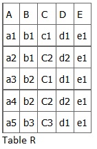
Figure 10.3 A relation table.
Unary Relational Operation: Selection
This is one of the operations developed specifically for relational databases. Recall that in SQL we were able to select which columns would appear in the output and we were able to use the WHERE clause to obtain a subset of the rows. In relational algebra, we would express this with the Greek letter σ and we use this to choose a subset of tuples from a relation that satisfies a selection condition.
Do not confuse the selection operator with the SQL key word “SELECT.” The former finds the tuples that satisfy a condition whereas the later determines which columns will be selected from the source database tables.
Figure 10.4 shows two selection queries in both SQL and relational algebra.
|
Select the Employee tuples where the DepartmentID is 4 |
Select the Employee tuples where the Salary is greater than $30,000 |
|
SELECT * FROM Employees WHERE DepartmentID = ‘4’ |
SELECT * FROM Employees WHERE Salary > 30000 |
|
σDepartmentID = 4 (Employees) |
σSalary > 30000 (Employees) |
Figure 10.4 The differences between SQL command and relational algebra.
The relational algebra expression has the Greek letter and the table name on the line and the conditional (the WHERE clause) is written as a subscript. Figure 10.5 shows this approach in a large font size.
|
σ <selection condition as a subscript> (Relation or table, normal line) |
Figure 10.5 The syntax in large font..
We can use the Boolean words of AND and OR. We can use comparison operators (=, <, ≤, >, ≥,≠). Figure 10.6 shows how this could be done with the two selects from Figure 10.4.
|
Select the Employee tuples where the DepartmentID is 4 OR the Salary is greater than $30,000 |
|
SELECT * FROM Employees WHERE DepartmentID = ‘4’ AND Salary > 30000 |
|
σDepartmentID = 4 AND Salary < 30000 (Employees) |
Figure 10.6 An example of a compound SQL command with a WHERE clause and a compound clause in Relational Algebra
Relational algebra uses a shorthand:
- The individual tuple is written as “t.”
- The relation is written as “R.”
- The attribute is written as “Ai.”
- We can write this as t[Ai].
We use the term “unary,” because we are dealing with a single relation or table and we are looking at each tuple individually.
Look at this expression: |σc (R)| ≤ |R|
This is stating that the results of a selection will either be the whole table or a subset of the table. We can NEVER have a result set with more rows than what appeared in the original table. Again, we can NEVER have more columns than the original table.
Terms may be used to describe the behavior of the selection.
- Selectivity of the condition.
- The fraction of tuples selected by a selection condition.
- Commutative
- The sequence of the selects can be applied in any order.
- σ<Condition1> (σ<Condition2>) (R)) = σ<Condition2> (σ<Condition1>) (R))
- Cascade or sequence
- You could nest a query as done in commutative. Or you could express this as a conjunction (the key word AND).
- σ<Condition1> (σ<Condition2>) (R)) = σ<Condition2> AND<Condition1>) (R))
We can use an example to understand the foregoing better. Vancouver British Columbia is home to Douglas College and to other institutions. We wish to find those individuals who have a connection to Douglas College as active students.
- Commutative: You could select all persons with a connection to Douglas College, then select out a list of active students. Or you could select out all active students from all institutions, then select out those with a connection to Douglas College. The resulting set would be the same.
- Cascade or sequence: Use either commutative approach or you could select all persons with a connection to Douglas College and a status as active student. And the order does not matter.
Unary Relational Operation: Projection
Projection is one of the operations developed specifically for relational databases. Selection will return all of the columns in a table. Projection permits us to select some of the columns from a table. The SQL key word “SELECT” does the same thing.
|
We want just an employee’s last name, first name, and salary. |
|
SELECT LastName, FirstName, Salary FROM Employees |
|
π LastName, FirstName, Salary(Employees) |
Figure 10.7 An example of projection in Relational Algebra
Notice that the column names are written as subscripts.
The projection operator has some interesting behaviors. If non-key attributes are used, then duplicate tuples are possible. If a key is used, then duplicate tuples cannot happen.
In the formal relational model, duplicates are not permitted. In SQL, this is allowed. To have this behavior, we would use the key word DISTINCT. In some circles, this is called a multiset or a bag of tuples.
Since projection is a special form of selection, the selection traits are present too. The exception is the property of commutativity. We cannot change the ordering of the columns in the column name list and have the same results in the output.
Unary Relational Operation: Renaming
Renaming is one of the operations developed specifically for relational databases. We use this operator in order to rename the output columns. Recall from regular algebra how you could use an immediate variable.
|
Example of an Algebra Problem Using Immediate Variables. |
|
X + Y + Z Let A = X + Y Answer: A + Z |
Figure 10.8 An example of an algebra problem using an immediate variable
This is similar to software programming where a variable is declared to hold a temporary value. The following snippet of Java code shows how we can change the stored values.
- int A = 2;
- int B = 3;
- int C = 4;
- int temp;
- temp = A; // The variable temp is holding the value of 2.
- A = B; // The variable A has taken on the new value of 3.
- B = C; // The variable B has taken on the new value of 4.
- C = temp; // The variable C has taken on the new value of 2.
- System.out.println (“A is “ + A + “. B is “ + B + “. C is “ + C + “.”);
- The output string is: A is 3. B is 4. C is 2.
The variable temp preserves the value that was originally stored in the variable A. Otherwise, this value would be lost as soon as the value stored in B is sent to the variable A.
Consider the example of retrieving the first name, last name, and salary of all employees who work in department number 5.
We select all employees that work in department number 5. We limit the columns just to the first name, the last name, and the salary (via the projection operator). This could have been done in two steps. The output from the department number 5 employees would be stored in a temporary variable3. Then we would take that temporary variable and feed it to the column selecting SQL.
|
Using Renaming Command |
|
DEP5_EMPS <— σDepartmentID = 5 (Employees) RESULTS <— π FirstName, LastName, Salary (DEP5_EMPS ) |
Figure 10.9 An example of relational algebra using an immediate variable (DEPT_EMPS)
Notice that in relational algebra that we do not use the Greek letter rho (ϸ). Instead, we use the left pointing arrow with a long tail.
We use the Greek letter rho (ϸ) when we are discussing the options as for listing out the three forms of renaming:
ϸ S(B1, B2, …, Bn)(R) or ϸ S(R) or ϸ(B1, B2, …, Bn)(R)
- Where ϸ is the RENAME operator.
- Where S is the new relation name.
- Where B1, B2, .., Bn are the new attribute names.
A bit more explanation:
- ϸ S(B1, B2, …, Bn)(R) is renaming both the relation and its attributes
- ϸ S(R) is renaming only the relation
- ϸ(B1, B2, …, Bn)(R) is renaming the attributes.
How the attributes are ordered in the original relation is how the new attributes are ordered in the new relation.
Binary Relational Operation: Union and Intersection
Union and intersection are operations from set theory.
We have worked with the SQL union command. An example will show how this operator is used.
We wish to retrieve the Social Security numbers of all employees who either work in department 5 or directly supervise an employee who works in department 5.
We could do this with temporary results via renaming and a union operation.
Result1 ← π Ssn(DEP5_EMPS)
Result2 ← π Super_ssn(DEP5_EMPS)
Result ← Result1 U Result2
The union operation produces the tuples that are in either Result1 or Result2 or both while removing any duplicates.
The intersection operation produces the tuples that are in both.
In the relational database world, the two sets of tuples must be of the same type (union compatibility or type compatibility).
We formally express union compatibility or type compatibility thusly:
- Two relations R(A1, A2, …, An) and S(B1, B2, …, Bn) are said to be union compatible (or type compatible) if they have the same degree4 n and if dom(Ai) = dom(Bi) for 1 ≤ I ≤ n.
- This means that the two relations have the same number of attributes (columns) and each corresponding pair of attributes has the same domain.
Union and intersection are commutative operations.
- R ∪ S = S ∪ R
- R ∩ S = S ∩ R
Union and intersection are associative operations. The grouping of the operations does not matter:
- R ∪ (S ∪ T) = (R ∪ S) ∪ T
- R ∩ (S ∩ T) = (R ∩ S) ∩ T
Binary Relational Operation: Set Difference
Set difference operation is from set theory.
These are the tuples that are present in one relation, but not present in a second relation. We write this as R – S, which states that this includes all tuples that are in R, but are not in S.
The two relations must be union compatibility or type compatibility.
Commutative operations cannot be applied to a set difference action.
In mathematics, an operation could be rewritten in different ways. Consider the following:
- 9 times 10
- 9 + 9 + 9 + 9 + 9 + 9 + 9 + 9 + 9 + 9
- 10 + 10 + 10 + 10 +10 + 10 + 10 + 10 + 10
- 10 times 10 – 10
Prove to yourself that the answer for each line is 90.
In binary relations, you could do the same thing. You could rewrite an intersection action as a series of unions and set differences:
- R ∩ S = ((R ∪ S ) − (R −S )) − (S −R)
Binary Relational Operation: Cartesian Product
Cartesian product is an operation from set theory. This is also known as “cross product.” If we drop the requirement that a relation must be union compatible, then you could have an output that is larger than either relation. The result is a new element by combining every member tuple from one relation set with every member tuple from the other relation set. In formal expression, we would write this as:
- R(A1, A2, …, An) X S(B1, B2, …, Bm) is a relation Q with degree n + m attributes Q(A1, A2, …, An, B1, B2, …, Bm), in that order.
If you create a join command and leave off the WHERE clause, then the result would be a Cartesian product. Suppose we wanted to output a list of every female employee with their children. We would need to include a WHERE clause of the female employee’s company ID number from two tables (the Employees table and the Dependents table). If the WHERE clause is omitted, then the output would have EVERY dependent name combined with EVERY female employee. Clearly this is not very useful.
Is there a place for the Cartesian product? Yes. Suppose you are in your favorite breakfast café. The menu has two columns as shown in Figure 10.10:
|
Proteins |
Sides |
|
Chicken |
Mushroom Pasta |
|
Salmon |
Spinach and Mushrooms |
|
Cod |
Slaw |
|
Scallops |
Sun-dried tomatoes |
|
Octopus |
Arugula salad |
|
|
Broccoli |
Figure 10.10 An example of a menu with five proteins and six sides
You do not wish to eat the same combination twice in a 30-day period. Using mathematics, you know that 5 times 6 is 30. And you could work this out by hand:
|
Chicken |
Salmon |
Cod |
Scallops |
Octopus |
|
Mushroom Pasta |
Mushroom Pasta |
Mushroom Pasta |
Mushroom Pasta |
Mushroom Pasta |
|
Spinach and Mushrooms |
Spinach and Mushrooms |
Spinach and Mushrooms |
Spinach and Mushrooms |
Spinach and Mushrooms |
|
Slaw |
Slaw |
Slaw |
Slaw |
Slaw |
|
Sun-dried tomatoes |
Sun-dried tomatoes |
Sun-dried tomatoes |
Sun-dried tomatoes |
Sun-dried tomatoes |
|
Arugula salad |
Arugula salad |
Arugula salad |
Arugula salad |
Arugula salad |
|
Broccoli |
Broccoli |
Broccoli |
Broccoli |
Broccoli |
Figure 10.11 Working out by hand the 30 possible combinations
Using Cartesian product or leaving off the WHERE clause, the output would be as follows:
|
Chicken |
Mushroom Pasta |
|
Chicken |
Spinach and Mushrooms |
|
Chicken |
Slaw |
|
Chicken |
Sun-dried tomatoes |
|
Chicken |
Arugula salad |
|
Chicken |
Broccoli |
|
Salmon |
Mushroom Pasta |
|
Salmon |
Spinach and Mushrooms |
|
Salmon |
Slaw |
|
Salmon |
Sun-dried tomatoes |
|
Salmon |
Arugula salad |
|
Salmon |
Broccoli |
|
Cod |
Mushroom Pasta |
|
Cod |
Spinach and Mushrooms |
|
Cod |
Slaw |
|
Cod |
Sun-dried tomatoes |
|
Cod |
Arugula salad |
|
Cod |
Broccoli |
|
Scallops |
Mushroom Pasta |
|
Scallops |
Spinach and Mushrooms |
|
Scallops |
Slaw |
|
Scallops |
Sun-dried tomatoes |
|
Scallops |
Arugula salad |
|
Scallops |
Broccoli |
|
Octopus |
Mushroom Pasta |
|
Octopus |
Spinach and Mushrooms |
|
Octopus |
Slaw |
|
Octopus |
Sun-dried tomatoes |
|
Octopus |
Arugula salad |
|
Octopus |
Broccoli |
Figure 10.12 Using Cartesian product to obtain the 30 possible combinations
Binary Relational Operation: Join Operation
Join operation is an operation from set theory. A relational database is powerful, because of the ability to pull data from two or more tables. The output could have more fields or columns than one of the input tables. This is similar to the traits of a Cartesian product. The difference is that we use a WHERE clause to select out the useful rows.
As Thomas Connolly and Carolyn Begg pointed out:
- Join is one of the most difficult operations to implement efficiently in a… [relational] DBMS and is one of the reasons why relational systems have intrinsic performance problems.
Imagine that we wish to retrieve the name of each manager for each department in an organization. The Departments table contains the SSN for the manager. The Employees table contains the names of the managers. Recall that we used normalization and that is why the managers’ names and other details are not stored in the Departments table. The manager’s SSN is a foreign key in the Departments table. Here is the join command as expressed in relational algebra:
- DepartmentManager ←Departments ⋈ ManagerSSN=SSN Employees
This would create a long tuple. We can remove the unwanted columns by using projection:
- Result ←πDepartmentName, LastName, FirstName(DepartmentManager)
If the Departments table used “SSN” instead of “ManagerSSN,” then the line would appear as
- DepartmentManager ←Departments ⋈ Departments.SSN=Employees.SSNEmployees
Notice the table name, the period (the “dot”), and the field or column name.
According to Thomas Connoly and Carolyn Begg, there are five types of join operations
- Theta join
- Equijoin
- Natural join
- Outer join
- Semijoin
An inner join will return rows from two tables that satisfies a given condition. This is the most widely used join operation. An inner join can be divided into three sub types:
- Theta join
- Equijoin5
- Natural join
Theta Join
A theta join pulls from two tables based on a condition represented by the Greek letter theta (θ). θ could be any one of the comparison operators. The general form is:
|
Formal Form |
SQL Form |
|
R ⋈θ S6
|
SELECT <column names> FROM <first table name> INNER JOIN <second table name> ON <first table name column> = <second table name column> |
Figure 10.13 The formal form and the SQL form of a theta (θ) join.
To understand theta joins better, consider the following example:
|
TableA |
|
TableB |
||
|
Column1 |
Column2 |
|
Column1 |
Column2 |
|
1 |
1 |
|
1 |
1 |
|
1 |
2 |
|
1 |
3 |
Figure 10.14 The theta (θ) join example with two tables. Adapted from Fiona Brown’s example. (Corrected to conform with the Third Edition Style Guide.) Source: https://www.guru99.com/joins-sql-left-right.html
We will take R ⋈θ S and rewrite it as:
R ⋈ R.Column2 > S.Column2 (S)7
The output would be8
|
R ⋈ R.Column2 > S.Column2 (S) |
|
|
Column1 |
Column2 |
|
1 |
2 |
Figure 10.15 The theta (θ) join example output table. Adapted from Fiona Brown’s example. (Corrected to conform with the Third Edition Style Guide.) Source: https://www.guru99.com/joins-sql-left-right.html
This example is very simple and is a bit misleading. In a theta join (and in the equijoin), both columns that are mentioned in the conditional clause would appear in the output.
Equijoin
An equijoin is like a theta join in that the equijoin operation pulls from two tables based on a condition represented by the Greek letter theta (θ). But θ is the equal symbol (=). We will use the previous example to illustrate the equijoin.
R ⋈ R.Column2 = S.Column2 (S)
The output would be
|
R⋈R.Column2 = S.Column2 (S) |
|
|
Column1 |
Column2 |
|
1 |
1 |
Figure 10.16 The equijoin example output table. Adapted from Fiona Brown’s example. (Corrected to conform with the Third Edition Style Guide.) Source: https://www.guru99.com/joins-sql-left-right.html
Equijoin is not a SQL key word. The WHERE clause contains the equal symbol.
Natural Join
A natural join is like a theta join that pulls from two tables, but the extra column is not included in the output and the ON key word is not used. So in Figure 10.13, there would be no theta expression and there would be no ON clause.
Recall that in the union operation, the number of attributes must be the same and the domain types need to be the same. For the natural join, there is the additional requirement that the two tables share at least one common attribute. A natural join will match the common column values and eliminate any duplications. We will use a different example to illustrate a natural join.
|
Squares |
|
Cubes |
||
|
Number |
Square |
|
Number |
Cube |
|
2 |
4 |
|
2 |
8 |
|
3 |
9 |
|
3 |
18 |
Figure 10.17 The natural join example tables. Adapted from Fiona Brown’s example. (Corrected to conform with the Third Edition Style Guide.) Source: https://www.guru99.com/joins-sql-left-right.html
We would write the natural join as
|
Formal Expression |
SQL Expression |
|
Squares ⋈ Cubes
|
SELECT * FROM Squares NATUAL JOIN Cubes; |
Figure 10.18 The formal form and the SQL form of the natural join for Figure 10.17.
The output would be
|
Squares ⋈ Cubes |
||
|
Number |
Square |
Cube |
|
2 |
4 |
8 |
|
3 |
9 |
18 |
Figure 10.19 The example output table for the natural join. Adapted from Fiona Brown’s example. (Corrected to conform with the Third Edition Style Guide.) Source: https://www.guru99.com/joins-sql-left-right.html
Outer Joins
An outer join will return rows from two tables even if there are no matches in one of the tables. An outer join can be divided into three sub types:
The outer join is a join in which the tuples from one relation are included even though there is no match in the second relation.
Left Outer Join
For the left outer join, you could imagine that the main table is on the “left” and the second table is on the “right.” Figure 10.20 uses Venn diagrams to illustrate this operation:
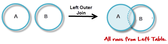
Figure 10.20 Venn diagrams illustrating a left outer join. Source of image: https://www.guru99.com/joins-sql-left-right.html
To see this from a different viewpoint, we will take the table from Figure 10.17 and add another row.
|
Squares |
|
Cubes |
||
|
Number |
Square |
|
Number |
Cube |
|
2 |
4 |
|
2 |
8 |
|
3 |
9 |
|
3 |
18 |
|
4 |
16 |
|
5 |
75 |
Figure 10.21 The source tables for the outer joins. Adapted from Fiona Brown’s example. (Corrected to conform with the Third Edition Style Guide.) Source: https://www.guru99.com/joins-sql-left-right.html
We would write the left outer join as
|
Formal Expression |
SQL Expression |
|
Squares ⟕ Cubes
|
SELECT <column names> FROM Squares LEFT OUTER12 JOIN Cubes ON Squares.Number = Cubes.Number |
Figure 10.22 The formal form and the SQL form of the left outer join for Figure 10.21.
The output would be
|
Squares ⟕ Cubes |
||
|
Number |
Square |
Cube |
|
2 |
4 |
8 |
|
3 |
9 |
18 |
|
4 |
16 |
NULL |
Figure 10.23 The example output table for the left outer join. Adapted from Fiona Brown’s example. (Corrected to conform with the Third Edition Style Guide.) Source: https://www.guru99.com/joins-sql-left-right.html
Again, all of the Squares table rows are included in the output plus any matching rows from the Cubes table rows. Any “missing” rows in this table are noted as NULLs.
If you only want the columns from the left table, then you would use the semijoin.
Right Outer Join
For the right outer join, you could imagine that the main table is on the “right” and the second table is on the “left.” Figure 10.24 uses Venn diagrams to illustrate this operation:
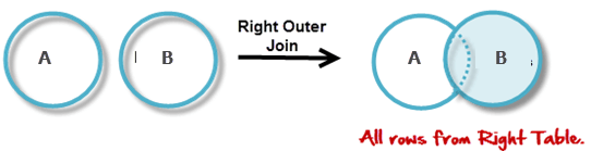
Figure 10.24 Venn diagrams illustrating a right outer join. Source of image: https://www.guru99.com/joins-sql-left-right.html
To see this from a different viewpoint, we will take the table from Figure 10.17.
We would write the right outer join as
|
Formal Expression |
SQL Expression |
|
Squares ⟖ Cubes
|
SELECT <column names> FROM Cubes RIGHT OUTER13 JOIN Squares ON Cubes.Number = Squares.Number |
Figure 10.25 The formal form and the SQL form of the right outer join for Figure 10.17.
The output would be
|
Squares ⟖ Cubes |
||
|
Number |
Cube |
Square |
|
2 |
8 |
4 |
|
3 |
18 |
9 |
|
5 |
75 |
NULL |
Figure 10.26 The example output table for the right outer join. Adapted from Fiona Brown’s example. (Corrected to conform with the Third Edition Style Guide.) Source: https://www.guru99.com/joins-sql-left-right.html
Again, all of the Cubes table rows are included in the output plus any matching rows from the Squares table rows. Any “missing” rows in this table are noted as NULLs.
Full Outer Join
For the full outer join, you could imagine that there are two main tables and we are including all tuples or rows in the output. It seems that we are ignoring the matching condition clause. That is not true. This helps to determine where the NULL entries would appear. Figure 10.27 uses Venn diagrams to illustrate this operation:
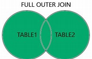
Figure 10.27 Venn diagrams illustrating a full outer join. Source of image: https://www.w3schools.com/sql/sql_join_full.asp14
To see this from a different viewpoint, we will take the table from Figure 10.17.
We would write the full outer join as
|
Formal Expression |
SQL Expression |
|
Squares ⟗ Cubes
|
SELECT <column names> FROM Squares FULL OUTER15 JOIN Cubes ON Squares.Number = Cubes.Number |
Figure 10.28 The formal form and the SQL form of the right outer join for Figure 10.17.
The output would be
|
Squares ⟗ Cubes |
||
|
Number |
Square |
Cube |
|
2 |
4 |
8 |
|
3 |
9 |
18 |
|
4 |
16 |
NULL |
|
5 |
NULL |
75 |
Figure 10.29 The example output table for the full outer join. Adapted from Fiona Brown’s example. (Corrected to conform with the Third Edition Style Guide.) Source: https://www.guru99.com/joins-sql-left-right.html
Again, all of the rows from both tables are included in the output with “missing” fields filled in as NULLs.
Other Joins
The inner join is the most widely used join operation and can be regarded as the default join type. We have explored the theta join, the natural join, and equijoin. These are “short cut” ways of expressing a desired form of the inner join.
Outer joins preserve rows with incomplete data. For example, we could see in the output both customers that have ordered something and that have not ordered anything recently.
Some databases support the self join. This is when one table is treated as two tables. W3 schools website has an example where the user is looking for customers that are from the same city. The syntax is a bit odd. See https://www.w3schools.com/sql/sql_join_self.asp for this example
The anti join will return the rows that semi join had rejected. See https://blog.dailydoseofds.com/p/what-are-semi-anti-and-natural-joins for more information.
Figure 10.30 shows seven of the possible joins.
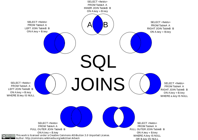
Figure 10.30 Seven join SQL commands with Venn diagrams. Source of image: https://www.techdoge.in/2017/10/learn-sql-MySql-what-is-join-and-how-to-use-them.html
Binary Relational Operation: Division
The division operation is defined to be a relation over the attributes that consists of the set of tuples from R that match the combination of every tuple in S. This abstract definition may be hard to understand. The following are example use cases where the division operator would be useful:
- Find suppliers that can provide all parts.
- Find all employees who have worked on all projects controlled by one department.
- Find the topic that is taught in all courses.
Do not confuse regular algebra subtraction and division. For example:
10 / 2 is similar to 10 – 2 becomes 8 -2 becomes 6 – 2 becomes 4 – 2 becomes 2 – 2, which is subtracting the number 2 five times.
In relational algebra subtraction, we are looking for all tuples that are present in the first table, but are not in the second table. In relational algebra division, we are looking for something in the first table that has a relationship with every entity in the second table.
Imagine that you have come to the British Columbia government website that has a list of post-secondary institutions (https://www2.gov.bc.ca/gov/content/education-training/post-secondary-education/find-a-program-or-institution/find-an-institution). Behind the page, imagine that there are two database tables. One contains all of the possible academic majors available in British Columbia. The second table contains rows that have the institution’s name and the available academic majors. Figure 10.31 shows an extract from these imaginary database tables.
|
MajorsInBC |
|
InstitutionsAndMajors |
|
|
AvailableMajors |
|
Institution |
Majors |
|
Computer Application Training |
|
British Columbia Institute of Technology |
Computer Application Training |
|
Computer Hardware |
|
British Columbia Institute of Technology |
Computer Hardware |
|
Forensic Computing |
|
British Columbia Institute of Technology |
Forensic Computing |
|
Networking and Security |
|
British Columbia Institute of Technology |
Networking and Security |
|
Software Development |
|
British Columbia Institute of Technology |
Software Development |
|
Web Technologies |
|
British Columbia Institute of Technology |
Web Technologies |
|
Computing Studies and Information Systems |
|
Camosun College |
Marketing |
|
Web and Mobile Computing |
|
Camosun College |
Sport Management |
|
Fine and Applied Arts |
|
Capilano University |
Fine and Applied Arts |
|
Global and Community Studies |
|
Capilano University |
Global and Community Studies |
|
General Studies |
|
Coast Mountain College |
General Studies |
|
Marketing |
|
Coast Mountain College |
Environmental Geoscience Specialization |
|
Sport Management |
|
Douglas College |
Computing Studies and Information Systems |
|
Environmental Geoscience Specialization |
|
Douglas College |
Web and Mobile Computing |
Figure 10.31 Data drawn from the British Columba education website and from several institutions in British Columbia.
Figure 10.31 does not list all 25 higher education institutions in British Columbia. Nor does Figure 10.31 list all of the possible majors the sample institutions or the rest of the higher education institutions. Let’s imagine that you wish to explore all web computing programs.
We could use MajorsInBC ÷ InstitutionsAndMajors. The result would be as follows:
|
InstitutionsAndMajors |
|
|
British Columbia Institute of Technology |
Web Technologies |
|
Douglas College |
Web and Mobile Computing |
|
= |
|
|
MajorsInBC |
|
|
Web |
|
Figure 10.32 Result of finding institutions in British Columbia with a web major.16
This contrived example ignored the fact that “web technologies” and “web and mobile computing” are different. The problem with this example is that the second table is not normalized.
Some textbooks and some websites do not address this topic. Most SQL implementations do not support the division operation. So how would division be done in modern relational DBMS?
The Geeks for Geeks article listed the following ways to implement relational division in SQL:
- Method 1: Use cross join and EXCEPT
- Method 2: Use correlated subquery and NOT EXISTS
As division can be rendered as a series of subtraction steps, relational algebra can do the same thing:
- Generate all combinations by computing the Cartesian product of all possible y values in S with distinct x values in R.
- Identify the incomplete combinations. Use the subtract relational operator by subtracting R from the combinations in step 1 in order to find x values not associated with every y.
- Subtract the identified x values from all x values to get those associated with every y.
One final note. It is possible to use the regular division operator in SQL17. An example might be that you wish to output what would be value of dividing in half the current price of products in a table.
SELECT Price, Price / 2 AS “Half Price”
FROM Products;
This is not the relational algebra division operator.
Regular Calculus and Relational Calculus
Regular calculus is the study of rates of change. Differential calculus is concerned with the rate of change and works with derivatives and differentials. There is great interest in the slope of a line. Integral calculus seeks to find the quantity where the rate of change is known. Integral calculus looks at the space or area under the curve or slope.
Wolfram MathWorld used the word “analysis” as another term for the word “calculus18.” Thomas Connoly and Carolyn Begg pointed out that relational calculus is closer to predicate calculus.
A predicate is an expression of one or more variables for a certain domain. Consider the following:
Douglas College is a public college.
Predicate calculus would make the following statements:
- “… is a public college” is a predicate and “Douglas College” is the subject.
- Let “Douglas College” be denoted as “x” and “..is a public college” be denoted as Predicate P. Then we can write
- P(x)
A predicate must have at least one object that is associated with the predicate. “Douglas College” is the required object.
We will not go any deeper on the topic of predicate calculus. You can learn more about this topic by visiting https://www.tutorialspoint.com/the-predicate-calculus
Relational calculus specifies what is to be retrieved whereas relational algebra states how to obtain the results. In relational calculus, we work with tuple relational calculus and with domain relational calculus.
Tuple Relational Calculus
In tuple relational calculus, we wish to obtain those tuples that are true for a certain predicate. Using the above predicate example (“Douglas College is a public college.”), we could use the following shorthand:
PublicCollege(S)
Where the tuple variable S would be the range of permitted values.
So we could have the following query:
Find the set of all tuples S such that F(S) is true
{S | F(S)|
Our S could be all public colleges in British Columbia, or in Canada, or in North America, or in the world. In this example, S would not contain high schools or people’s names or animal names.
In the above shorthand expression, the letter “F” is called a formula or in pure mathematical logic, a well-formed formula or wff.
Imagine that we are working with a database table with the names of Staffers and that contains the following columns:
- ID
- FirstName
- LastName
- Position
- Gender
- DoB
- Salary
- BranchNumber
We wish to express in relational calculus the following:
Find the ID, FirstName, LastName, Position, Gender, DoB, Salary, and BranchNumber for individuals earning more than $10,000.
This query would appear as follows:
{S | Staffers(s) ∧19 S.Salary > 10000}
The letter “S” between the left curved brace and the pipe symbol means all columns. The ∧ is the logical conjunction and may be read as “and.” This is the Boolean AND operator. A tuple is collected if the row exists with a Salary greater than $10,000. In this example, we are assuming that the Staffers table has only columns for ID, FirstName, LastName, Position, Gender, DoB, Salary, and BranchNumber. If we wish to select a subset such as the Salary column, then we would need to modify the last expression as follows:
{S.Salary | Staffers(s) ∧ S.Salary > 10000}
Predicate calculus uses two quantifiers. Relational calculus uses these same two quantifiers.
- The existential quantifier ∃20 means “there exists”. At least one instance or tuple is true for the statement.
- The universal quantifier ∀21 means “for all.” All tuples must be true for the statement.
Let’s use Douglas College as our example and express two statements in relational calculus:
- There exists a Course (C) tuple that has the same ID (CourseID) as the CourseID of the current Student tuple, S, and is located in New Westminster.
- Student(S) ∧ (∃C) (Course(C) ∧ (C.ID = S.CourseID) ∧ C.City = “New Westminster”
- For all Computing Studies and Information Systems courses (C), the city is New Westminster.
- (∀C) (C.City = “New Westminster”)
Negations could be used. So the last expression could be written as
Recall that the intersection binary relational operator could be rewritten as a series of union and set differences, so relational calculus statements could be expressed in other ways. De Morgan’s laws can be used. The following is another version of the last expression:
- ~(∃C) (C.City = “Coquitlam”)
Recall that in a Boolean environment, you could negate an AND statement by negating each element and changing the AND to become an OR:
~(A AND B) is the same thing as ~ A OR ~B23
This behavior is true in relational calculus. Notice the change in from ∀ to ∃.
You need to be careful, because you could create an unsafe expression. Look at the following:
- The set of all tuples that are not in the Student relation:
- {S | ~ Student(S)}
This is unsafe, because this would generate a huge number of tuples. To avoid this, we need to add a restriction that all values that appear in the result must be values in the domain of the expression E, donated as dom (E). Or to put it differently, the domain of E is the set of all values that appear explicitly in E or that appear in or more relations whose names appear in E. In the last relational calculus example, the domain of the expression is the set of all values that appear in the Student relation. So an expression is safe if all values that appear in the result are values drawn from the domain of the expression. All of the previous examples of tuple relational calculus are safe.
Domain Relational Calculus
Domain relational calculus uses variables, but the variables come the domains of the attributes instead from the tuples of relations. An expression in domain relational calculus has the following general form:
{ d1, d2, …, dn | F(d1, d2, …, dm) } m ≥ n
Where d1, d2, …, dn and d1, d2, …, dm represent the domain variables
Where F(d1, d2, …, dm) represents a formula composed of atoms and an atom has the one of the following forms:
-
-
- R(d1, d2, …, dn), where R is a relation of degree n and each di is a domain variable.
- di θ dj, where di and dj are domain variables and θ is one of the comparison operator (<, ≤, >, ≥, =, ≠); the domains di and dj must have members that can be compared by θ.
- di θ c,, where di is a domain variable, c is a constant from the domain of di, and θ is one of the comparison operators.
-
The word “atom” is used, because atoms are the building blocks for more complex formulae.
Recall the relational calculus example:
Find the ID, FirstName, LastName, Position, Gender, DoB, Salary, and BranchNumber for individuals earning more than $10,000.
That query appeared as follows:
{S | Staffers(s) ∧ S.Salary > 10000}
To demonstrate how complex a domain relational calculus expression can be, we will add the restriction of finding managers that earn more than $10,000. So this query would appear as follows:
{FirstName, LastName | ∃ID, Position, Gender, DoB, Salary, BranchNumber) (Staffers (ID, FirstName, LastName, Position, Gender, DoB, Salary, BranchNumber) ∧ Position = “Manager” ∧ Salary > 10000)}
The condition (Staffers (ID, FirstName, LastName, Position, Gender, DoB, Salary, BranchNumber) ensures that the domain variables are restricted to the attributes of the same tuple. Since we used this condition, we could use the shortcut of “Position = Manager” instead of “Staff.Position = “Manager.” This approach has an interesting benefit. We do not need to use the existential quantifier ∃. Another benefit is that these queries are safe.
Domain relational calculus was presented for completeness. We will not go any further.
Recapping Relational Algebra and Relational Calculus
Relational calculus specifies what is to be retried whereas relational algebra states how to obtain the results. For every relational algebra expression, there is an equivalent expression in relational calculus. And for every tuple relational calculus or domain relational calculus expression there is an equivalent relational algebra expression.
We can use the relational algebra to rewrite a query to be more efficient.
Relational algebra and relational calculus can be used to write statements as a common language (a lingua franca) between database developers. Consider the command for obtaining the first three rows from a database table:
- Microsoft: SELECT TOP 3 * FROM Customers;
- MySQL: SELECT * FROM Customers Limit 3;
- Oracle: SELECT * FROM Customers where rownum <= 3;
Key Terms
anti join: This will return the rows that semi join had rejected.
atom: This is a building block for more complex formulae in domain relational calculus.
binary: The operation involves two database tables.
Cartesian product: This is an operation from set theory. This is also known as “cross product.” If we drop the requirement that a relation must be union compatible, then you could have an output that is larger than either relation. The result is a new element by combining every member tuple from one relation set with every member tuple from the other relation set.
commutative: The sequence of actions could be changed and the answer would still be the same.
division: This operation is defined to be a relation over the attributes that consists of the set of tuples from R that match the combination of every tuple in S.
equijoin: This is like a theta join in that the equijoin operation pulls from two tables based on a condition represented by the Greek letter theta (θ). But θ is the equal symbol (=).
existential quantifier ∃: This means “there exists” at least one instance or tuple that is true for the statement.
intersection ∩: This is a set operation that does not have a counterpart in regular algebra. It extracts what is common to two database tables based on a conditional.
join ⋈: This is an operation from set theory. A way of pulling from two tables. This was added to the set operators.
natural join: This is like a theta join that pulls from two tables, but the extra column is not included in the output and the ON key word is not used.
operands: In regular algebra, these are variables or values used in an expression. In relational algebra, these are relations or variables that represent relations.
operators: In regular algebra, these are symbols that denote what will be done to the regular algebra operands. In relational algebra, these are the common actions that we need to do with relations in a database.
outer join: This will return rows from two tables even if there are no matches in one of the tables. An outer join can be divided into three sub types:
- Left outer join (R ⟕ S): Everything from left plus any matching rows on the left with the right table plus nulls for any missing rows.
- Right outer join (R ⟖ S): Everything from right plus any matching rows on the right with the left table plus nulls for any missing rows
- Full outer join (R ⟗ S): Everything from both tables plus nulls for any missing fields.
predicate: This is an expression of one or more variables for a certain domain. A predicate must have at least one object that is associated with the predicate.
projection π (The lower case Greek letter pi): This selects a subset of the available columns. This was added to the set operators.
relational algebra: This collects instances of relations as input and gives occurrences of relations as outputs. The expressions explain how to execute a query. The expressions are independent of any SQL system.
relational calculus: This specifies what is to be retrieved whereas relational algebra states how to obtain the results. In relational calculus, we work with tuple relational calculus and with domain relational calculus.
- Tuple relational calculus: This seeks to obtain those tuples that are true for a certain predicate. The variables come from the tuples of the relations.
- Domain relational calculus: This uses variables come from the domains of the attributes.
renaming ϸ (The lower case Greek letter rho): This renames the output columns. This was added to the set operators.
safe: The expression draws upon members of a defined domain.
self join: This is when one table is treated as two tables.
selection σ (The lower case Greek letter sigma): A way of selecting tuples that satisfies a selection condition. This was added to the set operators. Do not confuse this word with the SQL key word “SELECT,” which lists out the desired columns in the output.
selectivity of the condition: The fraction of tuples selected by a selection condition.
semijoin: In a left outer join, you would have the desired columns from both tables. Nulls would appear in the right hand table for missing values. A semijoin would drop the right-hand table’s columns. The result would be the tuples that have a match in the second table.
set difference: This is from set theory. These are the tuples that are present in one relation, but not present in a second relation. We write this as R – S, which states that this includes all tuples that are in R, but are not in S. The two relations must be union compatibility or type compatibility.
set operations: These are operations drawn from mathematical set theory. These are union, intersection, set difference, and Cartesian product.
theta join θ (The lower case Greek letter theta): This pulls from two tables based on a condition represented by the Greek letter theta (θ). θ could be any one of the comparison operators.
type compatibility: This states that the two database tables must have the same degree and the same domain. This is the same concept as is “union compatibility.”
unary: This means we are working with one relation or with one database table.
union ∪: This produces the tuples that are in either Result1 or Result2 or both while removing any duplicates. In the relational database world, the two sets of tuples must be of the same type (union compatibility or type compatibility).
union compatibility: This states that the two database tables must have the same degree and the same domain. This is the same concept as is “type compatibility.”
universal quantifier ∀: This means “for all.” All tuples must be true for the statement.
unsafe: The expression draws upon members outside of a defined domain.
Exercises
1. Explain what is the union operator and the SQL union action. Provide an example of the relational algebra expression and provide an example of the common SQL command. [CS2013 IM/RD 3, IM/RD 4; IT2017 ITE-IMA-05a.]
2. Explain what is the intersection operator. Provide an example of the relational algebra expression and provide an example of the common SQL command. [CS2013 IM/RD 3, IM/RD 4; IT2017 ITE-IMA-05a.]
3. Explain what is the difference operator. Provide an example of the relational algebra expression. Research your selected DBMS and find out if it supports the set difference operator. [CS2013 IM/RD 3, IM/RD 4; IT2017 ITE-IMA-05a.]
4. Explain what is the Cartesian product operator. Provide an informal example of when you might want to use the Cartesian product operator. [CS2013 IM/RD 3, IM/RD 4.]
5. Explain what is the select operator and the SELECT key word. Provide an example of the relational algebra expression and provide an example of the common SQL command. [CS2013 IM/RD 3, IM/RD 4; IT2017 ITE-IMA-05a.]
6. Explain what is the project operator and the SELECT key word. Provide an example of the relational algebra expression and provide an example of the common SQL command. [CS2013 IM/RD 3, IM/RD 4; IT2017 ITE-IMA-05a.]
7. Explain what is the join operator. Experts have different lists of the specialized join operators. List three joins that will provide tuples that satisfies only the conditional. List three joins that will include tuples with missing data. Provide an example of an inner join and provide an example of an outer join. Be sure to include both the formal form and the SQL form. There are 11 parts to this question. [CS2013 IM/RD 3, IM/RD 4; IT2017 ITE-IMA-05a.]
8. Explain what is the relational algebra division operator. Provide an informal example. [CS2013 IM/RD 3, IM/RD 4.]
9. Explain what is the natural join relational operator. Provide an example of the relational algebra expression and provide an example of the common SQL command. [IT2017 ITE-IMA-05a.]
10. Write queries in the tuple relational calculus for the following:
a. List all hotels
b. List all single rooms with a price below $200 per night.
c. List the names and cities of all guests.
d. List the price and type of all rooms at the Greenbrier Hotel.
A Running Project
Continue to work on your project.
Attribution
This chapter of Database Design is a brand-new addition.
This chapter drew from many sources.
Image Attributions
No second edition images were used.
References
Fiona Brown. “DBMS Joins: Inner, THETA, Outer, Equi Types of Join Operations,” Guru99, June 28, 2024. https://www.guru99.com/joins-sql-left-right.html
Thomas Connolly and Carolyn Begg. Database Systems: A Practical Approach to Design, Implementation, and Management, Addison Wesley, 2002, page 88.
“SQL | Division,” Geeks for Geeks, July 3, 2024. https://www.geeksforgeeks.org/sql-division/