Sampling
A Sampling Distribution Example
Learning Objectives
Calculate the typical metrics for sampling distribution problems.
Let us better understand sampling distributions with an example. We will do several probability calculations related to the example in the sections below.
Example 46.1
Problem Setup: The Canadian Internet Standards Group studies the use of the internet across Canada by various industries and demographics. They have recently published data stating that:
- Canadians 18 years of age and older spend on average 180 hours each year using the internet.
- The number of hours spent on the internet is highly skewed to the right with a standard deviation of 90 hours.
- A random sample of 64 adults is taken.
Part 1 - The Shape of the Distribution (Exercise)
Problem Setup: Let us continue with our example where:
- We sample 64 individuals
- They spend, on average 180 hours per year online
- With a standard deviation of 90 hours
- The number of hours is highly skewed right
Question: What is the shape of the distribution?
Part 2 - Greater Than Probability (Exercise)
Problem Setup: Let us continue with our example where:
- We sample 64 individuals
- They spend, on average 180 hours per year online
- With a standard deviation of 90 hours
- The number of hours is highly skewed right
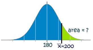
Question: What is the probability of our sample having a mean of greater than 200?
|
|
|
|
|
|
|
Click here to reveal the solutions to the above exercise.
Mean and Standard Error
- The mean of the sampling distribution is 180 hours or, [latex]\mu_{\bar{x}}= 180[/latex].
- The question is asking about the sample mean - it is not asking about any one individual Canadian 18 years of age or older
- The question is a sampling distribution question so we need to use the standard error formula.
- The standard error is [latex]\sigma_{\bar{x}}= 11.25[/latex] hours: \[ \sigma_{\bar{x}}= \frac{\sigma}{\sqrt{n}} = \frac{90}{\sqrt{64}} = 11.25 \text{ hours}\]
Graph of Area in Question
As with any other normal distribution problem, we start by drawing a distribution of the sampling distribution and label it appropriately with the information in the problem:
Excel Formula
To solve for the probability of the sample mean ([latex]\bar{x}[/latex]) being greater than 200 hours, we use the following Excel formula: \[ =1-\text{NORM.DIST}(200,180,11.25,1) = 0.0377 \].
Conclusion
There is a 3.77% chance that the sample average will be larger than 200 hours.
Part 3 - Less Than Probability (Exercise)
Problem Setup: Let us continue with our example where:
- We sample 64 individuals
- They spend, on average 180 hours per year online
- With a standard deviation of 90 hours
- The number of hours is highly skewed right
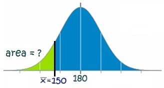
Question: What is the probability of our sample having a mean of less than 150?
Click here to reveal the solutions to the above exercise.
Mean and Standard Error
- The mean is the same as the previous example: [latex]\mu_{\bar{x}}= 180[/latex].
- Again, the question is asking about the sample mean and not about a particular individual so we are working with a sampling distribution question and need to use a standard error.
- The standard error is still [latex]\sigma_{\bar{x}}= 11.25[/latex] hours: \[ \sigma_{\bar{x}}= \frac{\sigma}{\sqrt{n}} = \frac{90}{\sqrt{64}} = 11.25 \text{ hours}\]
Graph of Area in Question
As with any other normal distribution problem, we start by drawing a distribution of the sampling distribution and label it appropriately with the information in the problem:
Excel Formula
To solve for the probability of the sample mean ([latex]\bar{x}[/latex]) being less than 150 hours, we use the following Excel formula: \[ =\text{NORM.DIST}(150,180,11.25,1) = 0.0038 \].
Conclusion
There is a 0.38% chance that the sample average will be less than 150 hours.
Part 4 - Within Probability (VIDEO)
Problem Setup: Let us continue with our example where:
- We sample 64 individuals
- They spend, on average 180 hours per year online
- With a standard deviation of 90 hours
- The number of hours is highly skewed right
Question: What is the probability of our sample mean being within 10 hours of the population mean?
Solution: Click here to download the Excel file shown in the video below.
Conclusion: There is a 62.6% chance that the sample mean is within 10 hours of the population mean.
Click here to expand written solutions to this problem
This question is asking the likelihood that the sample mean will be within 10 hours of the population - in other words, the probability that the sample mean will fall between -10 hours below the population mean to +10 hours above the population mean. This is illustrated as follows in Figure 46.3:
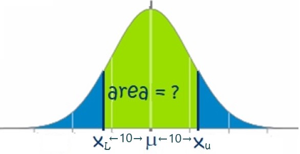
Here we only need to find the area on one side of the sampling distribution and then we can multiply it by 2 because we are dealing with a symmetrical distance of 10 hours above and below the population mean.
Using our sampling formula, we will determine the area between the center of the sampling distribution to a sample mean of 190 hours. Thus the numerator is +10 (i.e., the difference between the sample mean of 190 and the population mean of 180) and the corresponding z-score will be:
\[ Z = \frac{\bar{x}-\mu}{\sigma_{\bar{x}}} = \frac{10}{11.25} = 0.8889\]
Thus, we round up our z-score to 0.89 and look up the corresponding area on the cumulative standardized normal table. A z-score of 0.89 corresponds to an area of 0.8106.. This is the area that falls less than a sample mean of 190 hours. Thus, the area from the center of our sampling distribution to the sample mean of 190 hours is: [latex]0.8106 - 0.5 = 0.3106[/latex].
Next we must multiply this area by 2 because the question is asking about the likelihood of the sample mean being within 10 hours (i.e., on either side) of the population mean: [latex]0.3106 \times 2 = 0.6212[/latex]
Thus the likelihood of taking a sample of 64 adults and finding that they spend an average of 10 hours per year within the true population mean of 180 hours using the internet is 62.12% (quite likely!).
Part 5 - Inverse Sample Mean (VIDEO)
Problem Setup: Let us continue with our example where:
- We sample 64 individuals
- They spend, on average 180 hours per year online
- With a standard deviation of 90 hours
- The number of hours is highly skewed right
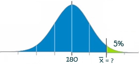
Question: What is the minimum sample mean that would be considered to be in the top 5% of internet users in Canada?
Solution: Click here to download the Excel file shown in the video below.
Conclusion: The minimum hours to be in the top 5% of internet users is 198.5 hours.
Click here to expand written solutions to this example
This question is asking us to determine the 95th percentile of the sample means with respect to the sampling distribution. In other words, what is value of the sample mean whereby 95% of all sample means fall less than this value (5% fall above this value).
We can illustrate this as follows in Figure 46.4:
Using our sampling formula, we know all everything except a z-score and the sample mean:
\[ Z = \frac{\bar{x}-\mu}{\sigma_{\bar{x}}} = \frac{\bar{x}-180}{11.25} \]
But recall, if we have an Area we can determine its corresponding z-score with the normal table. Thus, an area of 0.95 corresponds to the z-score of +1.645. We now have the following:
\[\frac{\bar{x}-180}{11.25} = 1.645\]
Solving for the sample mean we get: [latex]\bar{x} = 180 +1.645\cdot 11.25=198.51[/latex] hours hours (rounded to 2 decimal places). Thus 95% of all sample means will fall below 198.51 hours per year of internet use.
Your Own Notes (EXERCISE)
- Are there any notes you want to take from this section? Is there anything you'd like to copy and paste below?
- These notes are for you only (they will not be stored anywhere)
- Make sure to download them at the end to use as a reference
