<?xml version="1.0" encoding="UTF-8"?>
<!DOCTYPE html PUBLIC "-//W3C//DTD XHTML 1.1//EN" "http://www.w3.org/TR/xhtml11/DTD/xhtml11.dtd">
<html xmlns="http://www.w3.org/1999/xhtml" xml:lang="en">
<head>
<meta content="text/html; charset=UTF-8" http-equiv="content-type" />
<meta http-equiv="Content-Language" content="en" />
<meta name="generator" content="Pressbooks 4.4.0" />
<meta name="pb-author" content="Serhat Beyenir &amp; Sanja Boskovic" />
<meta name="pb-title" content="Simulator Laboratory" />
<meta name="pb-language" content="en-ca" />
<meta name="pb-cover-image" content="https://pressbooks.bccampus.ca/tpps/wp-content/uploads/sites/134/2017/03/PowerPlant.jpeg" />
<meta name="pb-subtitle" content="Sim Labs for Thermodynamics and Thermal Power Plant Simulator" />
<meta name="pb-copyright-year" content="2017" />
<meta name="pb-book-license" content="cc-by" />
<meta name="pb-about-140" content="Merging Theory with Practice: Sim Labs for Thermodynamics and Thermal Power Plant Simulator" />
<meta name="pb-about-50" content="Power and Process Engineering Program, School of Energy, BCIT" />
<meta name="pb-about-unlimited" content="This Simulator laboratory (SIMLAB) book was created to provide ancillary resources for Thermodynamics and Thermal Power Plant Simulator courses. It is intended to act as a collection of exercises to help our students merge the theory covered in the classroom with the practice performed in the labs." />
<meta name="pb-short-title" content="SIMLABS" />
<meta name="pb-primary-subject" content="TGMB" />
<meta name="pb-copyright-holder" content="Serhat Beyenir &amp; Sanja Boskovic" />
<meta name="pb-custom-copyright" content="Unless otherwise noted, this book is released under a Creative Commons Attribution (CC BY) 4.0 International license. Under the terms of the CC BY license you can freely share, copy or redistribute the material in any medium or format, or adapt the material by remixing, transforming or modifying this material providing you attribute Serhat Beyenir &amp; Sanja Boskovic. Attribution means you must give appropriate credit to Serhat Beyenir &amp; Sanja Boskovic as the original creator, note the CC BY license this document has been released under, and indicate if you have made any changes to the content. You may do so in any reasonable manner, but not in any way that suggests Serhat Beyenir &amp; Sanja Boskovic endorses you or your use of this work." />
<meta name="pb-author-file-as" content="Beyenir, Serhat and Boskovic, Sanja" />
<meta name="pb-additional-subjects" content="UYM" />
<meta name="pb-publisher" content="BCIT/BCcampus" />
<meta name="pb-publisher-city" content="Vancouver, B.C." />
<meta name="pb-publication-date" content="1512691200" />
<meta name="pb-keywords-tags" content="Thermodynamics, laboratory, simulator laboratory, Thermal Power Plant" />
<title>Simulator Laboratory</title>
</head>
<body lang='en'>
<div id="half-title-page"><h1 class="title">Simulator Laboratory</h1></div>
<div id="title-page"><h1 class="title">Simulator Laboratory</h1><h2 class="subtitle">Sim Labs for Thermodynamics and Thermal Power Plant Simulator</h2><h3 class="author">Serhat Beyenir &amp; Sanja Boskovic</h3><h4 class="contributing-authors"></h4><h4 class="publisher">BCIT/BCcampus</h4><h5 class="publisher-city">Vancouver, B.C.</h5></div>
<div id="copyright-page"><div class="ugc">
<div class="license-attribution" xmlns:cc="http://creativecommons.org/ns#"><p xmlns:dct="http://purl.org/dc/terms/"><a rel="license" href="http://creativecommons.org/licenses/by/4.0/"><img alt="Creative Commons License" style="border-width:0" src="https://i.creativecommons.org/l/by/4.0/88x31.png"></a><br><span property="dct:title">Simulator Laboratory</span> by Serhat Beyenir &amp; Sanja Boskovic is licensed under a <a rel="license" href="http://creativecommons.org/licenses/by/4.0/">Creative Commons Attribution 4.0 International License</a>, except where otherwise noted.</p></div>
<p><span itemscope="itemscope" itemtype="http://schema.org/Book" itemref="about alternativeHeadline author copyrightHolder copyrightYear datePublished description editor image inLanguage keywords publisher audience educationalAlignment educationalUse interactivityType learningResourceType typicalAgeRange">Unless otherwise noted, this book is released under a <a href="https://creativecommons.org/licenses/by/4.0/" target="_blank" rel="noopener">Creative Commons Attribution (CC BY) 4.0 International license</a>. Under the terms of the CC BY license you can freely share, copy or redistribute the material in any medium or format, or adapt the material by remixing, transforming or modifying this material providing you attribute Serhat Beyenir &amp; Sanja Boskovic. Attribution means you must give appropriate credit to Serhat Beyenir &amp; Sanja Boskovic as the original creator, note the CC BY license this document has been released under, and indicate if you have made any changes to the content. You may do so in any reasonable manner, but not in any way that suggests Serhat Beyenir &amp; Sanja Boskovic endorses you or your use of this work. </span></p></div></div>
<div class="front-matter dedication" id="dedication"><div class="front-matter-title-wrap"><h3 class="front-matter-number">1</h3><h1 class="front-matter-title">Dedication</h1></div><div class="ugc front-matter-ugc"><p>To our students who taught us to be better teachers than we were many years ago.</p> </div></div>
<div id="toc"><h1>Contents</h1><ul><li class="front-matter miscellaneous"><a href="#about-the-book"><span class="toc-chapter-title">About the Book</span></a></li><li class="front-matter image-credits"><a href="#attribution"><span class="toc-chapter-title">Credits</span></a></li><li class="front-matter preface"><a href="#preface"><span class="toc-chapter-title">Preface</span></a></li><li class="front-matter acknowledgements"><a href="#acknowledgments"><span class="toc-chapter-title">Acknowledgments</span></a></li><li class="part display-none"><a href="#sim-labs">Sim Labs</a></li><li class="chapter standard"><a href="#boiler-efficiency"><span class="toc-chapter-title">Boiler Efficiency</span></a></li><li class="chapter standard"><a href="#turbine-efficiency"><span class="toc-chapter-title">Turbine Efficiency</span></a></li><li class="chapter standard"><a href="#power-plant-efficiency"><span class="toc-chapter-title">Power Plant Efficiency</span></a></li><li class="chapter standard"><a href="#emissions-of-nox"><span class="toc-chapter-title">Emissions of NOx</span></a></li><li class="chapter standard"><a href="#heat-exchangers"><span class="toc-chapter-title">Heat Exchangers</span></a></li><li class="chapter standard"><a href="#combustion-analysis"><span class="toc-chapter-title">Combustion Analysis</span></a></li><li class="back-matter about-the-author"><a href="#authors"><span class="toc-chapter-title">Authors</span></a></li><li class="back-matter miscellaneous"><a href="#revision-history"><span class="toc-chapter-title">Revision History</span></a></li></ul></div>
<div class="front-matter miscellaneous" id="about-the-book"><div class="front-matter-title-wrap"><h3 class="front-matter-number">2</h3><h1 class="front-matter-title">About the Book</h1></div><div class="ugc front-matter-ugc"><p>These Simulator Laboratory Worksheets are open educational resources that align with BCIT&#8217;s Power Engineering Thermodynamics and Thermal Power Plant Simulator courses.</p> <p>Open educational resources (OER) are defined as “teaching, learning, and research resources that reside in the public domain or have been released under an intellectual property license that permits their free use and re-purposing by others.” (<a href="http://www.hewlett.org/programs/education/open-educational-resources" class="external-link" rel="nofollow">Hewlett Foundation</a>).</p> <p>Funding for this project was provided through an OER Grant from the <a href="http://open.bccampus.ca/" class="external-link" rel="nofollow">B.C. Open Textbook Project</a>. The B.C. Open Textbook Project began in 2012 with the goal of making post-secondary education in British Columbia more accessible by reducing student cost through the use of openly licensed textbooks and other OER. The B.C. Open Textbook Project is administered by BCcampus and funded by the <a href="http://www2.gov.bc.ca/gov/content/governments/organizational-structure/ministries-organizations/ministries/advanced-education-skills-training" class="external-link" rel="nofollow">British Columbia Ministry of Advanced Education, Skills and Training</a> and the <a href="http://www.hewlett.org/" class="external-link" rel="nofollow">Hewlett Foundation</a>.</p> <p>The BCcampus <a href="https://bccampus.ca/bccampus-editorial-guidelines-for-tone-voice-and-style/" class="external-link" rel="nofollow">Writing Guidelines for Style and Tone</a> were referenced during the copy editing and proof reading phases of this project and the <a href="https://en-ca.wordpress.org/plugins/pressbooks-textbook/" target="_blank" rel="noopener">Open Textbooks Theme</a> by Brad Payne was used in producing the book.</p> </div>
</div>
<div class="front-matter image-credits" id="attribution"><div class="front-matter-title-wrap"><h3 class="front-matter-number">3</h3><h1 class="front-matter-title">Credits</h1></div><div class="ugc front-matter-ugc"><p>Cover image by Gretar Ívarsson is found in the <a href="https://commons.wikimedia.org/w/index.php?curid=2523755">public domain</a>.</p> <p>Images of simulator user interface courtesy of <a href="https://kongsberg.com/kongsberg-digital/" target="_blank" rel="noopener">Kongsberg Digital Simulation</a>. We wish to thank Kongsberg for their continuous support.</p> </div>
</div>
<div class="front-matter preface" id="preface"><div class="front-matter-title-wrap"><h3 class="front-matter-number">4</h3><h1 class="front-matter-title">Preface</h1></div><div class="ugc front-matter-ugc"><p>There are certain theoretical concepts that power engineering students struggle with and there are limited number of textbooks or videos that address these concepts directly linked to the field of power engineering. When we present those challenging concepts in class we also want to make sure that our students develop safe working habits and environmental sensibilities related to sustainable operation of the power engineering equipment.</p> <p>The primary purpose of this project was to design and develop simulator lab worksheets (SIM LABS) that would be used as ancillary resources for Thermodynamics and Thermal Power Plant Simulator (TPPS) courses. We have limited time to teach theory and we also have to offer practical skills to our students, so having as many SIM LABS as possible can bring those challenging concepts closer to our students and enhance their hands-on skills.</p> <p>We consider this project as a first step to writing a comprehensive open textbook in the future. Through this project we aimed to</p> <ul><li>Involve our students in the creation of learning materials and increase their awareness of Open Educational Resources (OER) and Open Education in general,</li> <li>Create opportunities for collaboration: BCIT Marine Campus uses several simulators supplied by the same manufacturer as ours and the identical TPPS is utilized at Linnaeus University in Sweden. We hope this OER project will induce our colleagues here in Vancouver, B.C. and abroad to collaboration and consideration of OER in their teaching.</li> </ul> <p>A final note to instructors who teach similar courses: We will be glad to share the &#8220;Instructor Guides and Solutions&#8221; to all SIM LABS included in this booklet. Please email us at<br /> <a href="mailto:Sanja_Boskovic@bcit.ca">Sanja_Boskovic@bcit.ca</a> or <a href="mailto:Serhat_Beyenir@bcit.ca">Serhat_Beyenir@bcit.ca</a></p> </div>
</div>
<div class="front-matter acknowledgements" id="acknowledgments"><div class="front-matter-title-wrap"><h3 class="front-matter-number">5</h3><h1 class="front-matter-title">Acknowledgments</h1></div><div class="ugc front-matter-ugc"><p>We owe many thanks to Dr. David Porter (former Associate Vice President) for his leadership in open education during his short tenure at BCIT albeit very impactful. We are equally indebted to <a href="https://bccampus.ca/" target="_blank">BCcampus</a> and <a href="https://open.bcit.ca/" target="_blank">openBCIT</a> for co-sponsoring our project.</p> <p>This was a rare project in which we did not need to disentangle any bureaucratic red tape and that was due to rare people who were involved since day one of our work. Special thanks go to James Rout (Associate Vice President), Ken Jeffery and Lin Brander (co-chairs of the OpenEd Working Group) as well as Alison Griffin, Deirdre Grace, Holly Stanley and Rosario Passos in alphabetical order. These individuals kept us motivated and we truly appreciate their friendliness in equal measures.</p> <p>Also thanks to those whom we never met in person but received support within Open Grants.</p> <p>And last but not least, we would like to thank our students, the entire Class of 2017 for their hard work, cooperation and feedback: Adrian Pontellini, Amar Manhas, April Derald Burias, Asmamaw Gebremariam, Brodie Pulles, Chelsea  Chiao Shiun Lo, Cole Tewinkel, Darrick Cheung, Devin Hughes, Harjit Kang, Jesiah de Gouveia, John Aldana, Joshua Lewis, Kevin Hamann, Matthew Fermill, Nathan Kwong, Riley Walker, Ryan Ngun, Sean McGilp, Terence Ka Chun Pang, Tommy Yoo, Trevor Rigby, Tylar Hodson and Vangeli Asimakis.</p> </div>
</div>
<div class="chapter introduction standard" id="boiler-efficiency"><div class="chapter-title-wrap"><h3 class="chapter-number">1</h3><h2 class="chapter-title">Boiler Efficiency</h2></div><div class="ugc chapter-ugc"> <div class="bcc-box bcc-highlight"><h3>Learning Objectives</h3> <p>Operate the Plant in the following modes and compute the Boiler Thermal Efficiency</p> <ul><li>230 MW Burning HFO</li> <li>80% Load Burning Bio Fuel</li> <li>80% Load Burning Coal</li> <li>80% Load Burning Coal with soot built up.</li> </ul> </div> <h1>Theory</h1> <p>First we define efficiency. There are many ways to present it, for example, efficiency is the ability to do something without wasting energy, effort or time. Put it mathematically, it is the ratio of useful output to thermal energy input. Layperson often uses the terms efficiency and effectiveness interchangeably however efficiency is to do with minimizing waste and effectiveness to do with maximizing output (more on this in <a href="https://pressbooks.bccampus.ca/tpps/chapter/heat-exchangers/" target="_blank" rel="noopener">Heat Exchangers</a> Lab). Boiler efficiency is sometimes defined as combustion efficiency which is computed by the ratio of the burner’s capability to burn fuel completely to the unburnt fuel and excess air in the exhaust. Thermal efficiency on the other hand, indicates the heat exchanger&#8217;s (i.e. boiler&#8217;s) capacity to transfer heat from the combustion process to the water or steam in the boiler. In general, the maximum boiler efficiency attainable from a boiler depends on such factors as method of burning the fuel, design of the furnace and heat transfer surfaces. In addition, the type of fuel, boiler load and operational practices influence the boiler efficiency. In this lab, we focus on the fuel type, boiler load and best practices.</p> <h2>Boiler Thermal Efficiency</h2> <p>Next we express the Boiler Thermal Efficiency as follows:</p> <p style="text-align: center"><code><img src="https://s0.wp.com/latex.php?latex=%5Ceta_%7Bboiler%7D+%3D+%5Cfrac%7BEnergy%5C+to%5C+steam%7D%7BEnergy%5C+from%5C+fuel%7D&#38;bg=T&#38;fg=000000&#38;s=0&#38;zoom=1" alt="\eta_{boiler} = \frac{Energy\ to\ steam}{Energy\ from\ fuel}" title="\eta_{boiler} = \frac{Energy\ to\ steam}{Energy\ from\ fuel}" class="latex" /></code></p> <p>Where energy to steam is the heat transfer required to form steam. Let,</p> <p style="text-align: left">h<sub>2</sub>=specific enthalpy of steam formed, [kJ/kg],</p> <p style="text-align: left">h<sub>1</sub>=specific enthalpy of feed water, [kJ/kg].</p> <p>Because the steam is formed at constant pressure, heat transfer required to form 1 kg of steam in the boiler is</p> <p>Energy to Steam= (h<sub>2</sub>-h<sub>1</sub>) [kJ]</p> <p>Energy from fuel is computed from the mass of fuel used and its heat (calorific) value. For coal this is the heating value as measured in a bomb calorimeter and it corresponds to the internal energy of combustion. If</p> <p>m<sub>f</sub>= mass of fuel burned in a given time</p> <p>m<sub>s</sub>= mass of steam generated in the same time</p> <p>HV= heat value of fuel [kJ/kg]</p> <p>Energy from fuel= m<sub>f</sub> x HV [kJ]</p> <p>Then we can write:</p> <p style="text-align: center"><img src="https://s0.wp.com/latex.php?latex=%5Ceta_%7Bboiler%7D+%3D+%5Cfrac%7Bm_%7Bs%7D%28h_%7B2%7D-h_%7B1%7D%29%7D%7Bm_%7Bf%7DHV%7D100%5C%25&#38;bg=T&#38;fg=000000&#38;s=0&#38;zoom=1" alt="\eta_{boiler} = \frac{m_{s}(h_{2}-h_{1})}{m_{f}HV}100\%" title="\eta_{boiler} = \frac{m_{s}(h_{2}-h_{1})}{m_{f}HV}100\%" class="latex" /></p> <div class="textbox learning-objectives"><h3>Lab Instructions</h3> <p>You will run 4 different initial conditions in this lab:</p> <ul><li>I10 230 MW Burning HFO</li> <li>I15 80% Load Burning Bio Fuel</li> <li>I14 80% Load Burning Coal</li> <li>I14 80% Load Burning Coal and use MD250 to set up soot variables.</li> </ul> <p>For each condition collect the relevant data to compute the Boiler Thermal Efficiency.</p> </div> <h2 style="text-align: left">Hints &amp; Tips</h2> <p>For data collection, use trends as shown below:</p> <div id="attachment_57" style="max-width: 668px" class="wp-caption aligncenter"><a href="https://pressbooks.bccampus.ca/tpps/wp-content/uploads/sites/134/2017/03/Trends.jpg"><img src="https://pressbooks.bccampus.ca/tpps/wp-content/uploads/sites/134/2017/03/Trends.jpg" alt="Trends sample" class="size-full wp-image-57" width="658" height="520" srcset="https://pressbooks.bccampus.ca/tpps/wp-content/uploads/sites/134/2017/03/Trends.jpg 658w, https://pressbooks.bccampus.ca/tpps/wp-content/uploads/sites/134/2017/03/Trends-300x237.jpg 300w, https://pressbooks.bccampus.ca/tpps/wp-content/uploads/sites/134/2017/03/Trends-65x51.jpg 65w, https://pressbooks.bccampus.ca/tpps/wp-content/uploads/sites/134/2017/03/Trends-225x178.jpg 225w, https://pressbooks.bccampus.ca/tpps/wp-content/uploads/sites/134/2017/03/Trends-350x277.jpg 350w" /></a> <p class="wp-caption-text">Trends sample</p> </div> <p>In addition to various pressure, temperature and flow values, you will need to log the following tags in your trends:</p> <ul><li>H00810 HFO heat value</li> <li>H00870 Pellet heat value (bio fuel)</li> <li>H00830 Coal heat value</li> </ul> <p>To calculate the enthalpy values, you may use an app or online tool such as the Superheated Steam Table: <a href="https://goo.gl/GdVM4U" target="_blank" rel="noopener">https://goo.gl/GdVM4U</a></p> <p>For the coal operation with soot built up, use MD250 and set malfunctions as follows:</p> <div id="attachment_53" style="max-width: 632px" class="wp-caption aligncenter"><a href="https://pressbooks.bccampus.ca/tpps/wp-content/uploads/sites/134/2017/03/soot.jpg"><img src="https://pressbooks.bccampus.ca/tpps/wp-content/uploads/sites/134/2017/03/soot.jpg" alt="MD250 malfunction settings." class="size-full wp-image-53" width="622" height="311" srcset="https://pressbooks.bccampus.ca/tpps/wp-content/uploads/sites/134/2017/03/soot.jpg 622w, https://pressbooks.bccampus.ca/tpps/wp-content/uploads/sites/134/2017/03/soot-300x150.jpg 300w, https://pressbooks.bccampus.ca/tpps/wp-content/uploads/sites/134/2017/03/soot-65x33.jpg 65w, https://pressbooks.bccampus.ca/tpps/wp-content/uploads/sites/134/2017/03/soot-225x113.jpg 225w, https://pressbooks.bccampus.ca/tpps/wp-content/uploads/sites/134/2017/03/soot-350x175.jpg 350w" /></a> <p class="wp-caption-text">MD250 malfunction settings.</p> </div> <div class="textbox learning-objectives"><h3>Deliverables</h3> <p>Your lab report is to include the following:</p> <ul><li><strong>Trend plots:</strong> Supply all plots taken for each of the 4 conditions,</li> <li><strong>Computation:</strong> Use MATLAB or MS Excel and calculate the boiler thermal efficiency for the 4 conditions specified,</li> <li><strong>Conclusion:</strong> Write a summary (max. 500 words, in a text box if using Excel) comparing your results and suggestions for further study.</li> </ul> </div> <div class="textbox shaded"><p>Further Reading:</p> <ul><li>Fundamentals of Classical Thermodynamics SI Version by G. J. Van Wylen and R. E. Sonntag: Evaluation of Actual Combustion Processes.</li> <li>Thermal Engineering by H.L. Solberg, O.C. Cromer and A.R. Spalding: Capacity and Efficiency of Steam Generating Units.</li> <li>Basic Engineering Thermodynamics in SI Units by R. Joel: Boiler calculations.</li> </ul> </div> </div>
</div>
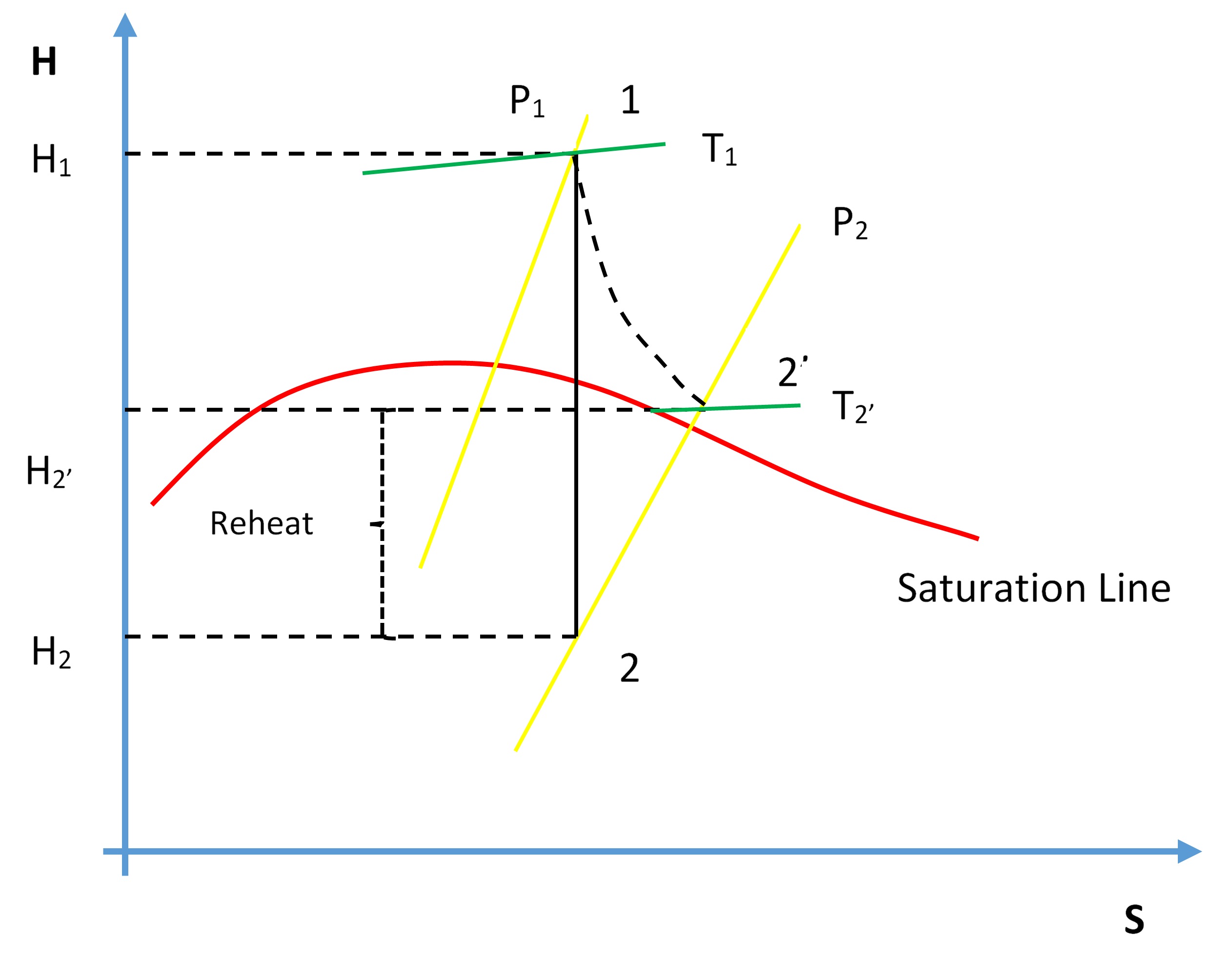
<div class="chapter standard" id="turbine-efficiency"><div class="chapter-title-wrap"><h3 class="chapter-number">2</h3><h2 class="chapter-title">Turbine Efficiency</h2></div><div class="ugc chapter-ugc"> <div class="bcc-box bcc-highlight"><h3>Learning Objectives</h3> <p>Operate the Plant at the following generating capacities to compute the isentropic change in enthalpy and thermal efficiency for the HP turbine.</p> <ul><li>35% Load (I13),</li> <li>80% Load (I14),</li> <li>230 MW (I10).</li> </ul> </div> <h1>Theory</h1> <p>Recall from the First and Second Law of Thermodynamics that the adiabatic process where entropy remains constant provides the maximum energy for work. As shown on the H-S coordinates, the difference in enthalpy, (H<sub>1</sub>-H<sub>2</sub>), is maximum when the lowest enthalpy (H<sub>2</sub>) is reached at the exit conditions. The ideal expansion is, therefore, a vertical line.</p> <div id="attachment_154" style="max-width: 2535px" class="wp-caption aligncenter"><a href="https://pressbooks.bccampus.ca/tpps/wp-content/uploads/sites/134/2017/03/HSDiagram.jpg"><img src="https://pressbooks.bccampus.ca/tpps/wp-content/uploads/sites/134/2017/03/HSDiagram.jpg" alt="Turbine efficiency." class="size-full wp-image-154" height="2005" width="2525" srcset="https://pressbooks.bccampus.ca/tpps/wp-content/uploads/sites/134/2017/03/HSDiagram.jpg 2525w, https://pressbooks.bccampus.ca/tpps/wp-content/uploads/sites/134/2017/03/HSDiagram-300x238.jpg 300w, https://pressbooks.bccampus.ca/tpps/wp-content/uploads/sites/134/2017/03/HSDiagram-768x610.jpg 768w, https://pressbooks.bccampus.ca/tpps/wp-content/uploads/sites/134/2017/03/HSDiagram-1024x813.jpg 1024w, https://pressbooks.bccampus.ca/tpps/wp-content/uploads/sites/134/2017/03/HSDiagram-65x52.jpg 65w, https://pressbooks.bccampus.ca/tpps/wp-content/uploads/sites/134/2017/03/HSDiagram-225x179.jpg 225w, https://pressbooks.bccampus.ca/tpps/wp-content/uploads/sites/134/2017/03/HSDiagram-350x278.jpg 350w" /></a> <p class="wp-caption-text">Turbine efficiency.</p> </div> <p>On the diagram above, T<sub>1</sub>, P<sub>1</sub> and P<sub>2</sub> are known process variables, for example, H<sub>1</sub> is determined by using T<sub>1</sub> and P<sub>1</sub>. H<sub>2</sub> then can be found drawing a vertical line from P<sub>1</sub> to P<sub>2</sub> by following adiabatic isentropic expansion (expansion at constant entropy).</p> <p>Non-ideal processes or real processes, however, do not present straight lines as shown on the Mollier diagram due to such factors as friction. If the expansion is not isentropic (i.e. entropy is not constant but it increases), the lowest enthalpy (H<sub>2</sub>) cannot be reached at the exit conditions, in other words, H<sub>2’</sub> &gt; H<sub>2</sub>. This means that ΔH for the ideal expansion is greater than ΔH for the non-ideal expansion between the same pressure boundaries. The internal turbine efficiency is therefore given by:</p> <p style="text-align: center"><code><img src="https://s0.wp.com/latex.php?latex=%5Ceta_%7BTurbine%7D+%3D+%5Cfrac%7BActual%5C+change%5C+in%5C+enthalpy%7D%7BIsentropic%5C+change%5C+in%5C+enthalpy%7D&#38;bg=T&#38;fg=000000&#38;s=0&#38;zoom=1" alt="\eta_{Turbine} = \frac{Actual\ change\ in\ enthalpy}{Isentropic\ change\ in\ enthalpy}" title="\eta_{Turbine} = \frac{Actual\ change\ in\ enthalpy}{Isentropic\ change\ in\ enthalpy}" class="latex" /></code></p> <p style="text-align: center"><img src="https://s0.wp.com/latex.php?latex=%5Ceta_%7BTurbine%7D+%3D+%5Cfrac%7B%28H_%7B1%7D-H_%7B2%5Cprime%7D%29%7D%7B%28H_%7B1%7D-H_%7B2%7D%29%7D&#38;bg=T&#38;fg=000000&#38;s=0&#38;zoom=1" alt="\eta_{Turbine} = \frac{(H_{1}-H_{2\prime})}{(H_{1}-H_{2})}" title="\eta_{Turbine} = \frac{(H_{1}-H_{2\prime})}{(H_{1}-H_{2})}" class="latex" /></p> <p>The difference in enthalpy H<sub>2’</sub>-H<sub>2</sub> is called the reheat factor and is the basis for multi-stage turbines. As can be seen on the Mollier diagram, the pressure curves are divergent. This means that the higher the pressure drop in a single stage turbine the greater the reheat factor and in turn the lower the turbine efficiency. However, if the steam is expanded through multiple stages and between each stage the steam is reheated, higher turbine efficiencies can be achieved. We will see this effect later in the <a href="https://pressbooks.bccampus.ca/tpps/chapter/power-plant-efficiency/" target="_blank" rel="noopener">Power Plant Efficiency</a> lab.</p> <div class="textbox learning-objectives"><h3>Lab Instructions</h3> <p><span itemscope="itemscope" itemtype="http://schema.org/WebPage"></span>You will run 3 different initial conditions in this lab:</p> <ul><li>35% Load (I13),</li> <li>80% Load (I14),</li> <li>230 MW (I10).</li> </ul> <p>For each condition collect the relevant data to compute the isentropic change in enthalpy for the HP turbine. Compare your results, which of the three conditions yield the most favourable results and why?</p> </div> <h2 style="text-align: left">Hints &amp; Tips</h2> <p>In addition to various pressure and temperature values; log the following tags in your trends:</p> <ul><li>Z03020</li> <li>E03018</li> </ul> <p>To calculate the enthalpy values, you may use an app or online tool such as the Superheated Steam Table: <a href="https://goo.gl/GdVM4U">https://goo.gl/GdVM4U</a></p> <div class="textbox learning-objectives"><h3>Deliverables</h3> <p>Your lab report is to include the following:</p> <ul><li><strong>Trend plots:</strong> Supply all plots taken for each of the 3 conditions,</li> <li><strong>Computation:</strong> Use MATLAB or MS Excel and calculate the turbine efficiency for the 3 conditions specified,</li> <li><strong>Conclusion:</strong> Write a summary (max. 500 words, in a text box if using Excel) comparing your results and suggestions for further study.</li> </ul> </div> <div class="textbox shaded"><p>Further Reading:</p> <ul><li><span itemscope="itemscope" itemtype="http://schema.org/WebPage">Thermodynamics and Heat Power by I. Granet: Vapor power cycles.</span></li> </ul> </div> </div>
</div>
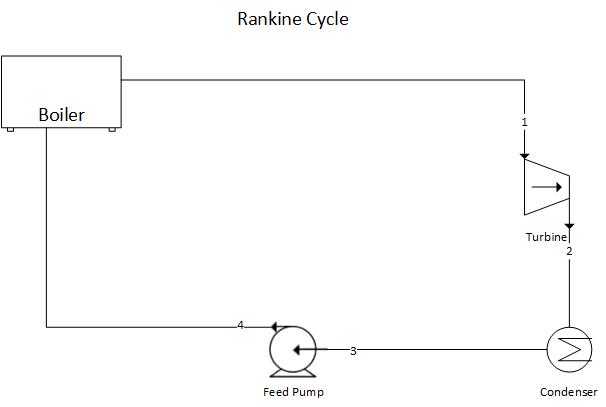
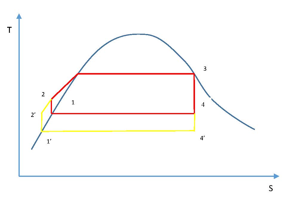
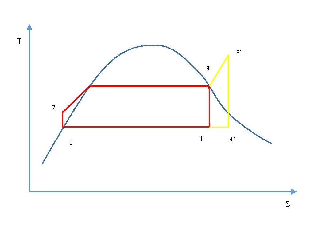
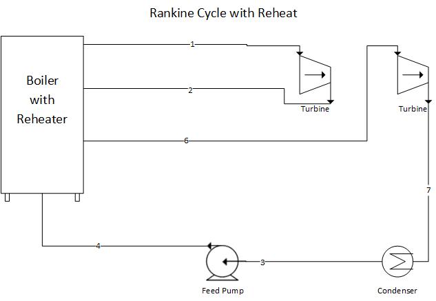
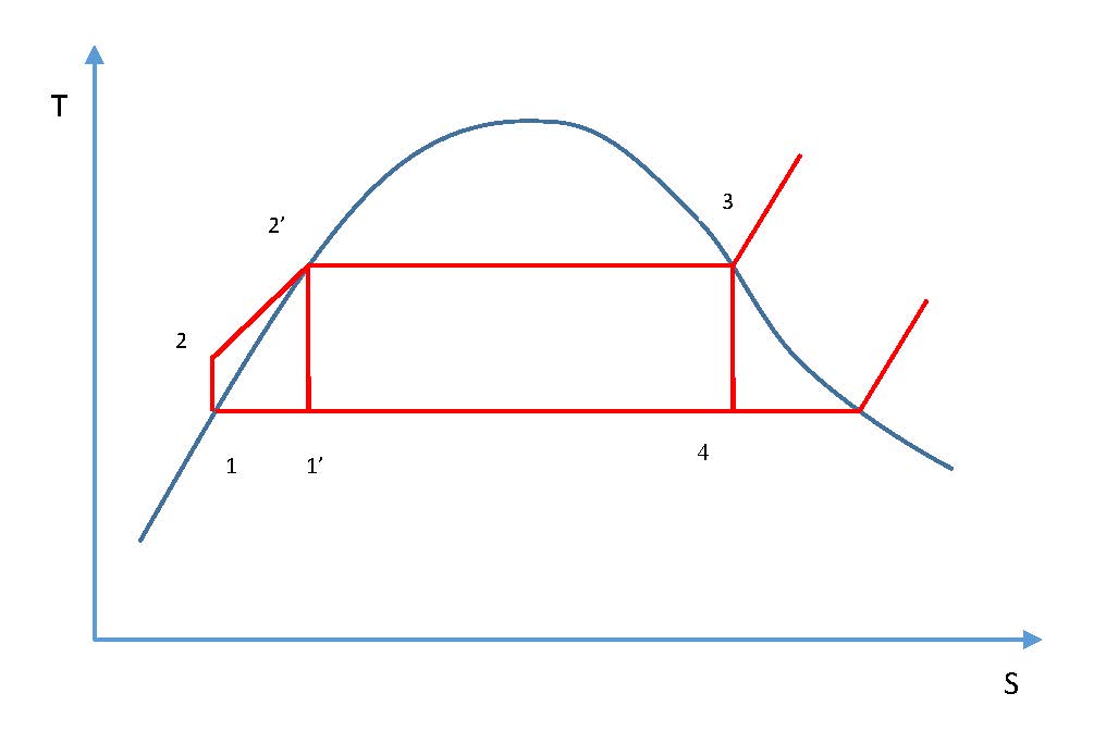
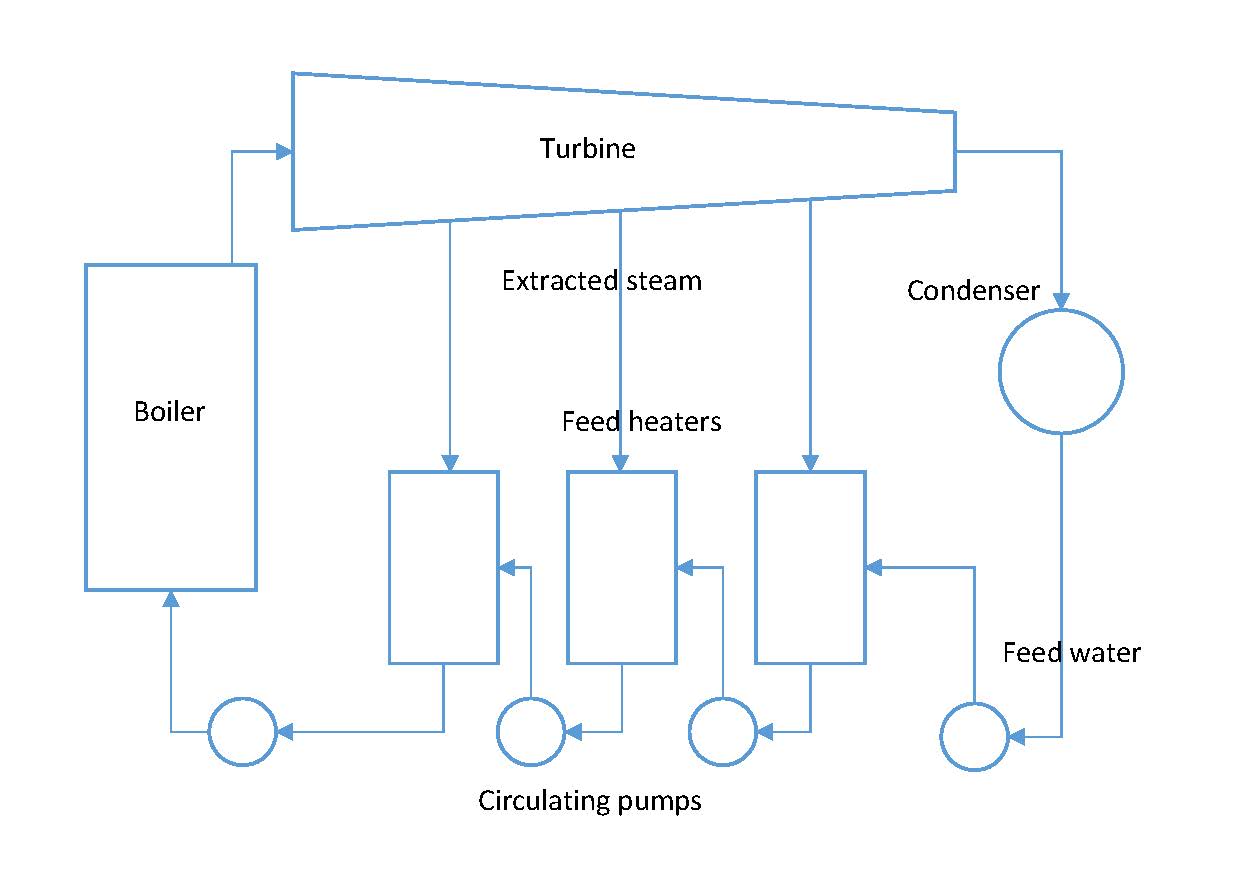
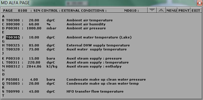
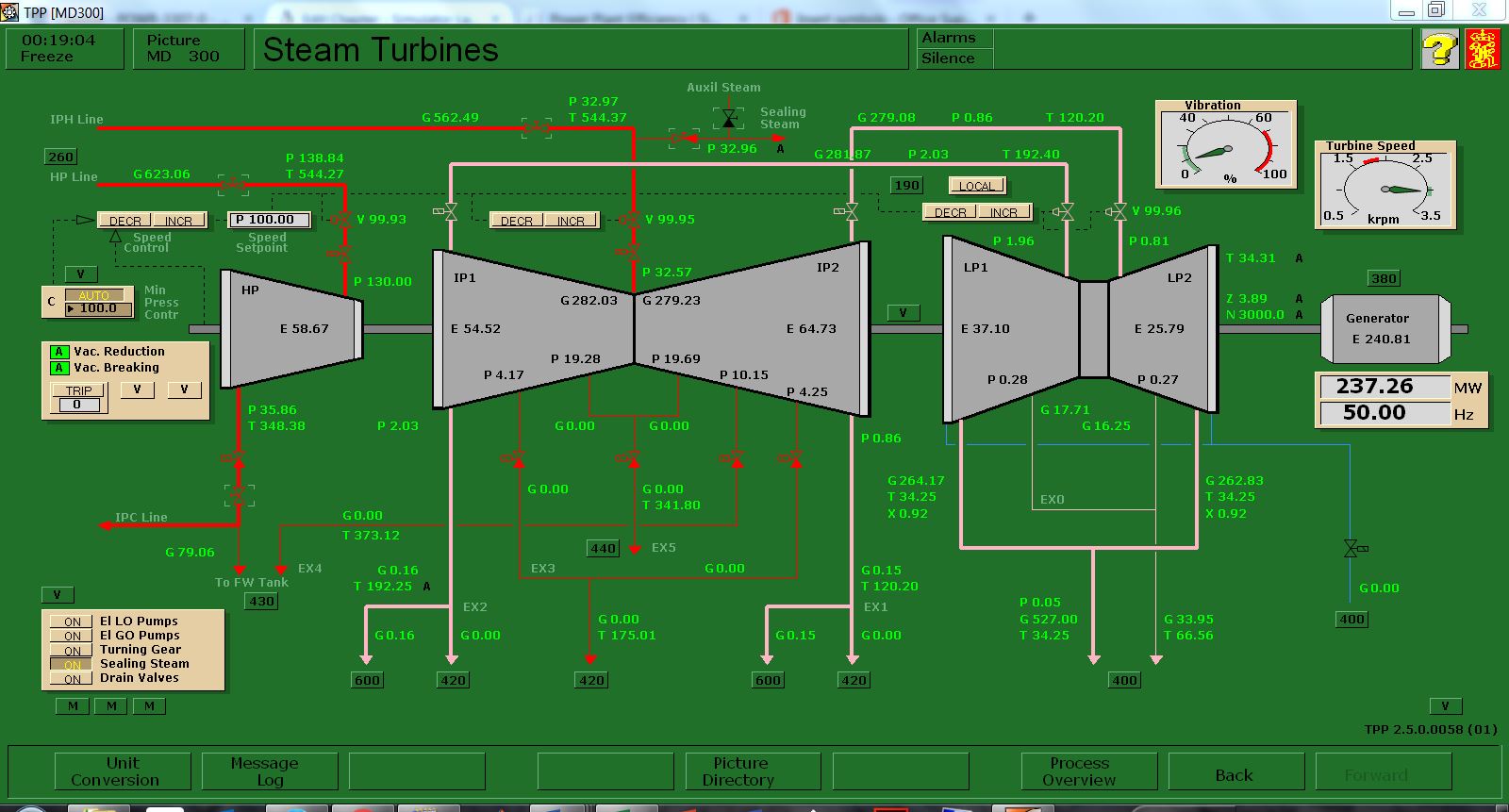
<div class="chapter standard" id="power-plant-efficiency"><div class="chapter-title-wrap"><h3 class="chapter-number">3</h3><h2 class="chapter-title">Power Plant Efficiency</h2></div><div class="ugc chapter-ugc"> <div class="bcc-box bcc-highlight"><h3>Learning Objectives</h3> <p>Operate the Plant at full generating capacity and compute the Power Plant Efficiency when the plant is operating:</p> <ul><li>Under normal conditions,</li> <li>With the cooling water temperature very high (lake water temperature: 35°C),</li> <li>Without regeneration.</li> </ul> </div> <h1>Theory</h1> <p>Excluding hydroelectric power plants, most power generating plants employ a type of boiler and steam turbine. A schematic diagram of a simple steam power plant is shown below:</p> <div id="attachment_50" style="max-width: 616px" class="wp-caption aligncenter"><a href="https://pressbooks.bccampus.ca/tpps/wp-content/uploads/sites/134/2017/03/RankineCycle.jpg"><img src="https://pressbooks.bccampus.ca/tpps/wp-content/uploads/sites/134/2017/03/RankineCycle.jpg" alt="Schematic diagram of a steam power plant" width="606" height="407" class="size-full wp-image-50" srcset="https://pressbooks.bccampus.ca/tpps/wp-content/uploads/sites/134/2017/03/RankineCycle.jpg 606w, https://pressbooks.bccampus.ca/tpps/wp-content/uploads/sites/134/2017/03/RankineCycle-300x201.jpg 300w, https://pressbooks.bccampus.ca/tpps/wp-content/uploads/sites/134/2017/03/RankineCycle-65x44.jpg 65w, https://pressbooks.bccampus.ca/tpps/wp-content/uploads/sites/134/2017/03/RankineCycle-225x151.jpg 225w, https://pressbooks.bccampus.ca/tpps/wp-content/uploads/sites/134/2017/03/RankineCycle-350x235.jpg 350w" /></a> <p class="wp-caption-text">Schematic diagram of a steam power plant</p> </div> <p>High-pressure steam leaves the boiler and enters the turbine. The steam expands in the turbine and does work which enables the turbine to drive the electric generator. The exhaust steam leaves the turbine and enters the condenser where heat is transferred from the steam to cooling water. The pressure of the condensate leaving the condenser is increased in the pump thereby enabling the condensate to flow into the boiler. This thermodynamic cycle is known as the Rankine Cycle.</p> <h2>The Rankine Cycle Efficiency</h2> <p>As noted above, some heat is always lost from the steam to cooling water. In addition, feed pumps consume energy thus reducing the net work output. Rankine Cycle Efficiency then can be expressed as:</p> <p style="text-align: center"><code><img src="https://s0.wp.com/latex.php?latex=%5Ceta_%7BRankine%7D+%3D+%5Cfrac%7BNet%5C+work%5C+output%7D%7BHeat%5C+supplied%5C+in%5C+the%5C+boiler%7D&#38;bg=T&#38;fg=000000&#38;s=0&#38;zoom=1" alt="\eta_{Rankine} = \frac{Net\ work\ output}{Heat\ supplied\ in\ the\ boiler}" title="\eta_{Rankine} = \frac{Net\ work\ output}{Heat\ supplied\ in\ the\ boiler}" class="latex" /></code></p> <p>or</p> <p style="text-align: center"><code><img src="https://s0.wp.com/latex.php?latex=%5Ceta_%7BRankine%7D+%3D+%5Cfrac%7BW_%7BTurbine%7D-W_%7BPump%7D%7D%7BQ_%7Bboiler%7D%7D&#38;bg=T&#38;fg=000000&#38;s=0&#38;zoom=1" alt="\eta_{Rankine} = \frac{W_{Turbine}-W_{Pump}}{Q_{boiler}}" title="\eta_{Rankine} = \frac{W_{Turbine}-W_{Pump}}{Q_{boiler}}" class="latex" /> </code></p> <p style="text-align: left">referring to the diagram above and using the enthalpy values in the Rankine cycle, we can write:</p> <p style="text-align: center"><code><img src="https://s0.wp.com/latex.php?latex=%5Ceta_%7BRankine%7D+%3D+%5Cfrac%7B%28h_%7B1%7D-h_%7B2%7D%29-%28h_%7B4%7D-h_%7B3%7D%29%7D%7B%28h_%7B1%7D-h_%7B4%7D%29%7D&#38;bg=T&#38;fg=000000&#38;s=0&#38;zoom=1" alt="\eta_{Rankine} = \frac{(h_{1}-h_{2})-(h_{4}-h_{3})}{(h_{1}-h_{4})}" title="\eta_{Rankine} = \frac{(h_{1}-h_{2})-(h_{4}-h_{3})}{(h_{1}-h_{4})}" class="latex" /></code></p> <h2>Improvements to the Rankine Cycle Efficiency</h2> <h3 style="text-align: left">Effect of Pressure and Temperature on the Rankine Cycle</h3> <p>If the exhaust pressure drops from P<sub>4</sub> to P<sub>4</sub>&#8216; with the corresponding decrease in temperature at which heat is rejected in the condenser the net work is increased by area 1-4-4&#8242;-1&#8242;-2&#8217;-2-1 (see diagram below)</p> <div id="attachment_58" style="max-width: 1008px" class="wp-caption aligncenter"><a href="https://pressbooks.bccampus.ca/tpps/wp-content/uploads/sites/134/2017/03/TS_ExhPress.jpg"><img src="https://pressbooks.bccampus.ca/tpps/wp-content/uploads/sites/134/2017/03/TS_ExhPress.jpg" alt="Effect of exhaust pressure" width="998" height="674" class="size-full wp-image-58" srcset="https://pressbooks.bccampus.ca/tpps/wp-content/uploads/sites/134/2017/03/TS_ExhPress.jpg 998w, https://pressbooks.bccampus.ca/tpps/wp-content/uploads/sites/134/2017/03/TS_ExhPress-300x203.jpg 300w, https://pressbooks.bccampus.ca/tpps/wp-content/uploads/sites/134/2017/03/TS_ExhPress-768x519.jpg 768w, https://pressbooks.bccampus.ca/tpps/wp-content/uploads/sites/134/2017/03/TS_ExhPress-65x44.jpg 65w, https://pressbooks.bccampus.ca/tpps/wp-content/uploads/sites/134/2017/03/TS_ExhPress-225x152.jpg 225w, https://pressbooks.bccampus.ca/tpps/wp-content/uploads/sites/134/2017/03/TS_ExhPress-350x236.jpg 350w" /></a> <p class="wp-caption-text">Effect of exhaust pressure</p> </div> <p>In a similar way, if the steam is superheated in the boiler, it is evident that the work is increased by area 3-3&#8242;-4&#8242;-4-3 (see diagram below):</p> <div id="attachment_60" style="max-width: 1059px" class="wp-caption aligncenter"><a href="https://pressbooks.bccampus.ca/tpps/wp-content/uploads/sites/134/2017/03/TS_Superheat.jpg"><img src="https://pressbooks.bccampus.ca/tpps/wp-content/uploads/sites/134/2017/03/TS_Superheat.jpg" alt="Effect of superheating" width="1049" height="745" class="size-full wp-image-60" srcset="https://pressbooks.bccampus.ca/tpps/wp-content/uploads/sites/134/2017/03/TS_Superheat.jpg 1049w, https://pressbooks.bccampus.ca/tpps/wp-content/uploads/sites/134/2017/03/TS_Superheat-300x213.jpg 300w, https://pressbooks.bccampus.ca/tpps/wp-content/uploads/sites/134/2017/03/TS_Superheat-768x545.jpg 768w, https://pressbooks.bccampus.ca/tpps/wp-content/uploads/sites/134/2017/03/TS_Superheat-1024x727.jpg 1024w, https://pressbooks.bccampus.ca/tpps/wp-content/uploads/sites/134/2017/03/TS_Superheat-65x46.jpg 65w, https://pressbooks.bccampus.ca/tpps/wp-content/uploads/sites/134/2017/03/TS_Superheat-225x160.jpg 225w, https://pressbooks.bccampus.ca/tpps/wp-content/uploads/sites/134/2017/03/TS_Superheat-350x249.jpg 350w" /></a> <p class="wp-caption-text">Effect of superheating</p> </div> <p>Superheating the steam is done by increasing the time the steam is exposed to the flue gases. The result of superheating is that for a given power output, the plant using superheated steam will be of smaller size than that using dry saturated steam.</p> <h3>The Reheat Cycle</h3> <p>Above we noted that the efficiency of the Rankine cycle is increased by superheating the steam. If metals could be found that would allow us to reach higher temperatures, the Rankine cycle could be more efficient. To improve the efficiency, the reheat cycle has been developed which is shown schematically below:</p> <div id="attachment_51" style="max-width: 643px" class="wp-caption aligncenter"><a href="https://pressbooks.bccampus.ca/tpps/wp-content/uploads/sites/134/2017/03/RankineCycleWithReheat.jpg"><img src="https://pressbooks.bccampus.ca/tpps/wp-content/uploads/sites/134/2017/03/RankineCycleWithReheat.jpg" alt="Rankine Cycle with Reheat" width="633" height="437" class="size-full wp-image-51" srcset="https://pressbooks.bccampus.ca/tpps/wp-content/uploads/sites/134/2017/03/RankineCycleWithReheat.jpg 633w, https://pressbooks.bccampus.ca/tpps/wp-content/uploads/sites/134/2017/03/RankineCycleWithReheat-300x207.jpg 300w, https://pressbooks.bccampus.ca/tpps/wp-content/uploads/sites/134/2017/03/RankineCycleWithReheat-65x45.jpg 65w, https://pressbooks.bccampus.ca/tpps/wp-content/uploads/sites/134/2017/03/RankineCycleWithReheat-225x155.jpg 225w, https://pressbooks.bccampus.ca/tpps/wp-content/uploads/sites/134/2017/03/RankineCycleWithReheat-350x242.jpg 350w" /></a> <p class="wp-caption-text">Rankine Cycle with Reheat</p> </div> <p>In this cycle, the steam is expanded to some intermediate pressure in the turbine and is then reheated in the boiler, after which it expands in the low-pressure turbine to the exhaust pressure. Rankine Cycle with reheat thermal efficiency can be expressed as:</p> <p style="text-align: center"><code><img src="https://s0.wp.com/latex.php?latex=%5Ceta_%7Bthermal%7D+%3D+%5Cfrac%7BW_%7B12%7D%2BW_%7B67%7D-W_%7B43%7D%7D%7BQ_%7B41%7D%2BQ_%7B26%7D%7D&#38;bg=T&#38;fg=000000&#38;s=0&#38;zoom=1" alt="\eta_{thermal} = \frac{W_{12}+W_{67}-W_{43}}{Q_{41}+Q_{26}}" title="\eta_{thermal} = \frac{W_{12}+W_{67}-W_{43}}{Q_{41}+Q_{26}}" class="latex" /> </code></p> <h3>The Regenerative Cycle</h3> <p>Another variation from the Rankine cycle is the regenerative cycle, which involves the use of feedwater heaters. During the process between states 2 and 2&#8242; the feedwater is heated and the average temperature is much lower during this process than during the vaporization process 2&#8242;-3. In other words, the average temperature at which heat is supplied in the Rankine cycle is lower than in the Carnot cycle 1&#8242;-2&#8242;-3-4-1&#8242;, and consequently the efficiency of the Rankine cycle is less than that of the corresponding Carnot cycle. The relationship between Carnot cycle and Rankine cycle is shown below.</p> <div id="attachment_59" style="max-width: 1026px" class="wp-caption aligncenter"><a href="https://pressbooks.bccampus.ca/tpps/wp-content/uploads/sites/134/2017/03/TS_Regen.jpg"><img src="https://pressbooks.bccampus.ca/tpps/wp-content/uploads/sites/134/2017/03/TS_Regen.jpg" alt="Relationship between Carnot cycle and Rankine cycle" width="1016" height="683" class="size-full wp-image-59" srcset="https://pressbooks.bccampus.ca/tpps/wp-content/uploads/sites/134/2017/03/TS_Regen.jpg 1016w, https://pressbooks.bccampus.ca/tpps/wp-content/uploads/sites/134/2017/03/TS_Regen-300x202.jpg 300w, https://pressbooks.bccampus.ca/tpps/wp-content/uploads/sites/134/2017/03/TS_Regen-768x516.jpg 768w, https://pressbooks.bccampus.ca/tpps/wp-content/uploads/sites/134/2017/03/TS_Regen-65x44.jpg 65w, https://pressbooks.bccampus.ca/tpps/wp-content/uploads/sites/134/2017/03/TS_Regen-225x151.jpg 225w, https://pressbooks.bccampus.ca/tpps/wp-content/uploads/sites/134/2017/03/TS_Regen-350x235.jpg 350w" /></a> <p class="wp-caption-text">Relationship between Carnot cycle and Rankine cycle</p> </div> <p>In the regenerative cycle, feedwater enters the boiler at some point between 2 and 2&#8242;. As a result, the average temperature at which heat is supplied is increased. A schematic of practical cycle is shown below:</p> <div id="attachment_52" style="max-width: 1254px" class="wp-caption aligncenter"><a href="https://pressbooks.bccampus.ca/tpps/wp-content/uploads/sites/134/2017/03/Regen.jpg"><img src="https://pressbooks.bccampus.ca/tpps/wp-content/uploads/sites/134/2017/03/Regen.jpg" alt="Regenerative cycle" width="1244" height="894" class="size-full wp-image-52" srcset="https://pressbooks.bccampus.ca/tpps/wp-content/uploads/sites/134/2017/03/Regen.jpg 1244w, https://pressbooks.bccampus.ca/tpps/wp-content/uploads/sites/134/2017/03/Regen-300x216.jpg 300w, https://pressbooks.bccampus.ca/tpps/wp-content/uploads/sites/134/2017/03/Regen-768x552.jpg 768w, https://pressbooks.bccampus.ca/tpps/wp-content/uploads/sites/134/2017/03/Regen-1024x736.jpg 1024w, https://pressbooks.bccampus.ca/tpps/wp-content/uploads/sites/134/2017/03/Regen-65x47.jpg 65w, https://pressbooks.bccampus.ca/tpps/wp-content/uploads/sites/134/2017/03/Regen-225x162.jpg 225w, https://pressbooks.bccampus.ca/tpps/wp-content/uploads/sites/134/2017/03/Regen-350x252.jpg 350w" /></a> <p class="wp-caption-text">Regenerative cycle</p> </div> <h2>The Plant Thermal Efficiency</h2> <p>In order to calculate the overall plant thermal efficiency, we need to adjust the formulas above to incorporate heat added in the reheater sections of the boiler:</p> <p style="text-align: center"><code><img src="https://s0.wp.com/latex.php?latex=%5Ceta_%7Bthermal%7D+%3D+%5Cfrac%7BW_%7BTurbines%7D-W_%7BPumps%7D%7D%7BQ_%7Bboiler%7D%2BQ_%7BReheat1%7D%2BQ_%7BReheat2%7D%7D&#38;bg=T&#38;fg=000000&#38;s=0&#38;zoom=1" alt="\eta_{thermal} = \frac{W_{Turbines}-W_{Pumps}}{Q_{boiler}+Q_{Reheat1}+Q_{Reheat2}}" title="\eta_{thermal} = \frac{W_{Turbines}-W_{Pumps}}{Q_{boiler}+Q_{Reheat1}+Q_{Reheat2}}" class="latex" /> </code></p> <div class="textbox learning-objectives"><h3>Lab Instructions</h3> <p>Run the initial condition I10 230 MW_oil_auto:</p> <ul><li>Draw a T-S diagram of the Rankine cycle (not to scale) including reheat and regeneration,</li> <li>Using Trend Group Directory, collect the relevant process values,</li> <li>Calculate the overall thermal efficiency of the plant: <ul><li>Under normal conditions,</li> <li>When the cooling water temperature is very high (Set the Variable List Page 0100, tag#: T00305 to 35°C),</li> <li>When all the steam extraction valves are closed (i.e. no regeneration and T00305 set to 10°C).</li> </ul> </li> </ul> </div> <h2 style="text-align: left">Hints &amp; Tips</h2> <p>In this lab, you are essentially calculating the Rankine Cycle thermal efficiency. However, you need to take the reheat cycle into consideration and log the following tags in your trends:</p> <ul><li>Q02395 Reheater 1 transferred heat</li> <li>Q02375 Reheater 2 transferred heat</li> </ul> <p>For Boiler Feedwater Inlet Temperature, you may use the Startup Heat Exchanger Feedwater Outlet Temperature tag#: T02447.</p> <p>For the second calculation, locate the Variable List Page 0100 as shown below:</p> <div id="attachment_44" style="max-width: 721px" class="wp-caption aligncenter"><a href="https://pressbooks.bccampus.ca/tpps/wp-content/uploads/sites/134/2017/03/LakeWaterTemp.jpg"><img src="https://pressbooks.bccampus.ca/tpps/wp-content/uploads/sites/134/2017/03/LakeWaterTemp.jpg" alt="Lake water temperature setting" width="711" height="351" class="size-full wp-image-44" srcset="https://pressbooks.bccampus.ca/tpps/wp-content/uploads/sites/134/2017/03/LakeWaterTemp.jpg 711w, https://pressbooks.bccampus.ca/tpps/wp-content/uploads/sites/134/2017/03/LakeWaterTemp-300x148.jpg 300w, https://pressbooks.bccampus.ca/tpps/wp-content/uploads/sites/134/2017/03/LakeWaterTemp-65x32.jpg 65w, https://pressbooks.bccampus.ca/tpps/wp-content/uploads/sites/134/2017/03/LakeWaterTemp-225x111.jpg 225w, https://pressbooks.bccampus.ca/tpps/wp-content/uploads/sites/134/2017/03/LakeWaterTemp-350x173.jpg 350w" /></a> <p class="wp-caption-text">Lake water temperature setting</p> </div> <p>For the third calculation, make sure you closed all steam extraction valves and set T00305 to 10°C:</p> <div id="attachment_45" style="max-width: 1610px" class="wp-caption aligncenter"><a href="https://pressbooks.bccampus.ca/tpps/wp-content/uploads/sites/134/2017/03/NoExtraction.jpg"><img src="https://pressbooks.bccampus.ca/tpps/wp-content/uploads/sites/134/2017/03/NoExtraction.jpg" alt="No steam extraction" width="1600" height="861" class="size-full wp-image-45" srcset="https://pressbooks.bccampus.ca/tpps/wp-content/uploads/sites/134/2017/03/NoExtraction.jpg 1600w, https://pressbooks.bccampus.ca/tpps/wp-content/uploads/sites/134/2017/03/NoExtraction-300x161.jpg 300w, https://pressbooks.bccampus.ca/tpps/wp-content/uploads/sites/134/2017/03/NoExtraction-768x413.jpg 768w, https://pressbooks.bccampus.ca/tpps/wp-content/uploads/sites/134/2017/03/NoExtraction-1024x551.jpg 1024w, https://pressbooks.bccampus.ca/tpps/wp-content/uploads/sites/134/2017/03/NoExtraction-65x35.jpg 65w, https://pressbooks.bccampus.ca/tpps/wp-content/uploads/sites/134/2017/03/NoExtraction-225x121.jpg 225w, https://pressbooks.bccampus.ca/tpps/wp-content/uploads/sites/134/2017/03/NoExtraction-350x188.jpg 350w" /></a> <p class="wp-caption-text">No steam extraction</p> </div> <p>To calculate the enthalpy values, you may use an app or online tool such as the Superheated Steam Table: <a href="https://goo.gl/GdVM4U" target="_blank" rel="noopener">https://goo.gl/GdVM4U</a></p> <div class="textbox learning-objectives"><h3>Deliverables</h3> <p>Your lab report is to include the following:</p> <ul><li><strong>T-S diagram:</strong> As per instructions above,</li> <li><strong>Trend plots:</strong> Supply all plots taken for this lab,</li> <li><strong>Computation:</strong> Use MATLAB or MS Excel and calculate the overall thermal efficiency of the plant as per Lab Instructions.</li> <li><strong>Conclusion:</strong> Write a summary (max. 500 words, in a text box if using Excel) comparing your results and suggestions for further study.</li> </ul> </div> <div class="textbox shaded"><p>Further Reading:</p> <ul><li>Applied Thermodynamics for Engineering Technologists by T. D. Eastop and A. McConkey: Steam Plant.</li> <li>Fundamentals of Classical Thermodynamics SI Version by G. J. Van Wylen and R. E. Sonntag: Vapor power cycles.</li> <li>Thermodynamics and Heat Power by I. Granet: Vapor power cycles.</li> </ul> </div> </div>
</div>
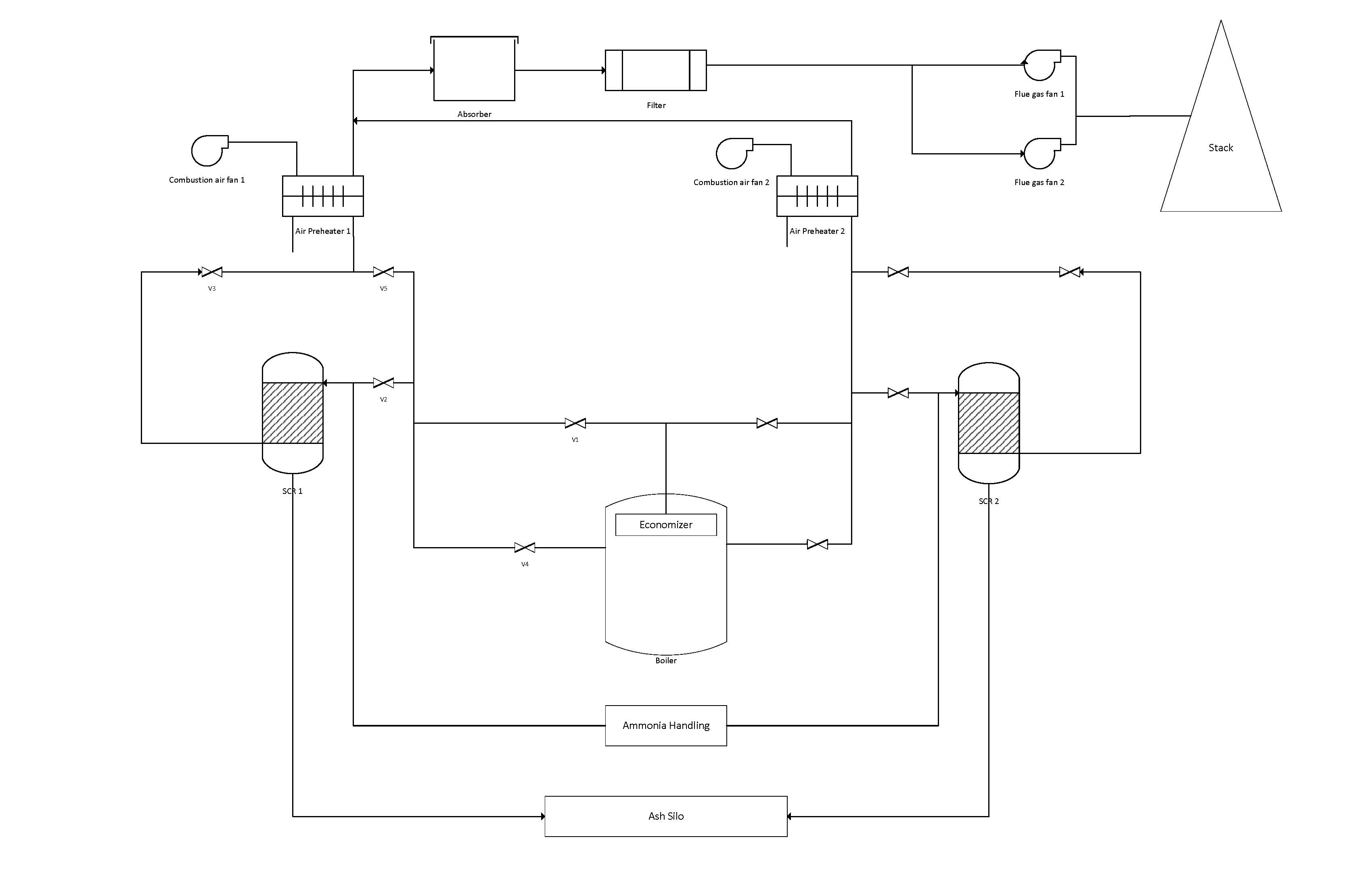
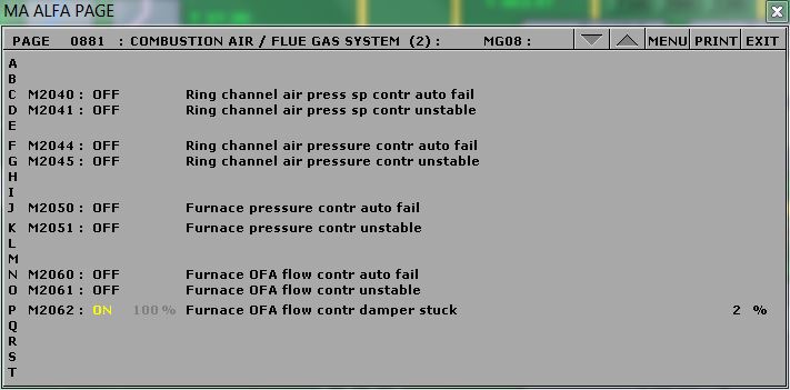
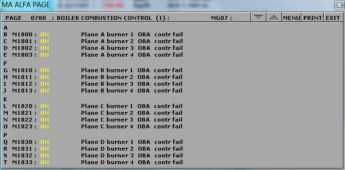
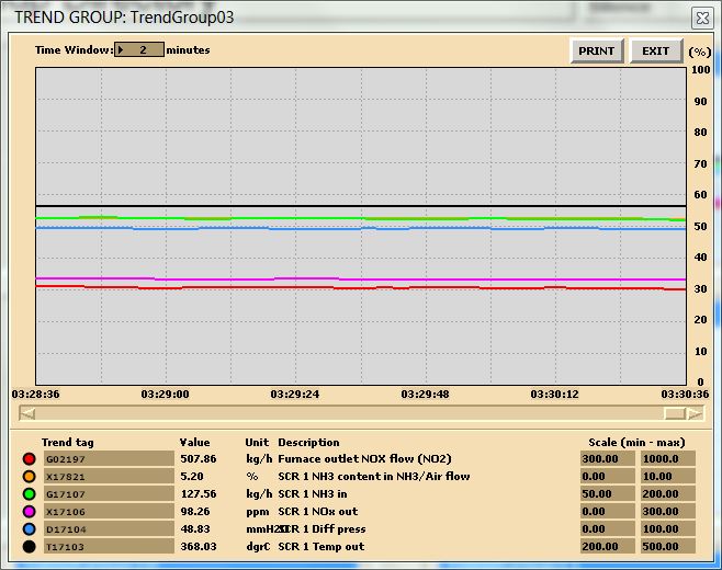
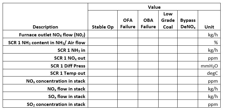
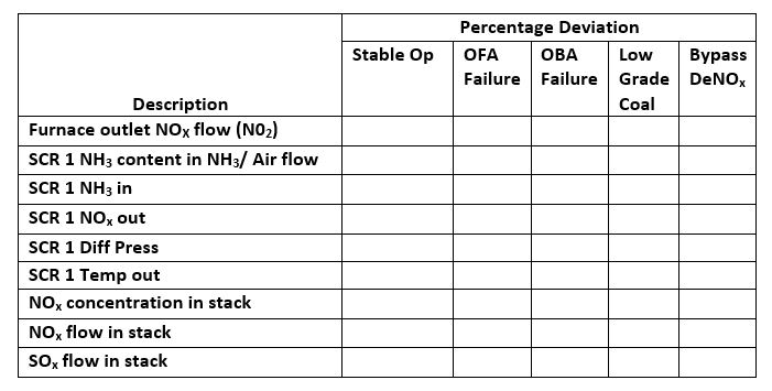
<div class="chapter standard" id="emissions-of-nox"><div class="chapter-title-wrap"><h3 class="chapter-number">4</h3><h2 class="chapter-title">Emissions of NOx</h2></div><div class="ugc chapter-ugc"> <div class="bcc-box bcc-highlight"><h3>Learning Objectives</h3> <p>Operate the Plant at full generating capacity and compare the NO<sub>x</sub> emissions when the plant is operating:</p> <ul><li>Under normal conditions,</li> <li>During over fire air damper failure,</li> <li>During over burner air control failure,</li> <li>Burning poor quality fuel,</li> <li>With the DeNO<sub>x</sub> plant bypassed.</li> </ul> </div> <h1>Theory</h1> <p>Combustion of coal generates considerable quantities of byproducts, some of which are considered pollutants. The byproducts are mostly water vapor which is what we see coming out of a power plant smokestack, carbon dioxide, and nitrogen that is readily available in the air we breathe, and they do not necessarily pose any direct health hazard. However, the emissions do carry small concentrations of pollutants into the atmosphere, which translate into large quantities of hazardous emissions due to the large amount of coal combusted. The main pollutants that can cause health problems are sulfur oxides, nitrogen oxides, particulate matter (see <a href="https://pressbooks.bccampus.ca/tpps/chapter/combustion-analysis/" target="_blank">Combustion Analysis</a>) and such trace elements as arsenic, lead and mercury.</p> <p>During the combustion process in a coal-fired power plant, nitrogen from the coal and air is converted into nitric oxide (NO) and nitrogen dioxide (NO<sub>2</sub>); these nitrogen oxides are commonly known as NO<sub>x</sub>. NO<sub>x</sub> emissions contribute to the formation of acid rain.</p> <p>NO<sub>x</sub> is primarily formed by two mechanisms: thermal NO<sub>x</sub> and fuel-bound NO<sub>x</sub>.</p> <p>Thermal NO<sub>x</sub> formation takes place at high flame temperatures. Formation of thermal NO<sub>x</sub> increases exponentially with combustion temperature. Fuel-bound NO<sub>x</sub> formation is dependent upon the nitrogen content of the fuel.</p> <p>The best way to minimize NO<sub>x</sub> formation is to reduce flame temperature, reduce excess oxygen, and/or to burn low nitrogen-containing fuels.</p> <h2>The DeNO<sub>x</sub> Plant Description</h2> <p>The purpose of the DeNO<sub>x</sub> plant is for removal of nitrogen oxide from the flue gases. The plant employs a selective catalytic reduction method. The medium used for the reduction is ammonia gas.</p> <p>The DeNO<sub>x</sub> plant includes two selective catalytic reduction (SCR) reactors and an ash silo. Various dampers channel the flue gases either into or bypass the SCR-reactors.</p> <div id="attachment_238" style="max-width: 3410px" class="wp-caption aligncenter"><a href="https://pressbooks.bccampus.ca/tpps/wp-content/uploads/sites/134/2017/03/DeNOxPlantOverview.jpg"><img src="https://pressbooks.bccampus.ca/tpps/wp-content/uploads/sites/134/2017/03/DeNOxPlantOverview.jpg" alt="DeNOxPlantOverview" class="size-full wp-image-238" width="3400" height="2200" srcset="https://pressbooks.bccampus.ca/tpps/wp-content/uploads/sites/134/2017/03/DeNOxPlantOverview.jpg 3400w, https://pressbooks.bccampus.ca/tpps/wp-content/uploads/sites/134/2017/03/DeNOxPlantOverview-300x194.jpg 300w, https://pressbooks.bccampus.ca/tpps/wp-content/uploads/sites/134/2017/03/DeNOxPlantOverview-768x497.jpg 768w, https://pressbooks.bccampus.ca/tpps/wp-content/uploads/sites/134/2017/03/DeNOxPlantOverview-1024x663.jpg 1024w, https://pressbooks.bccampus.ca/tpps/wp-content/uploads/sites/134/2017/03/DeNOxPlantOverview-65x42.jpg 65w, https://pressbooks.bccampus.ca/tpps/wp-content/uploads/sites/134/2017/03/DeNOxPlantOverview-225x146.jpg 225w, https://pressbooks.bccampus.ca/tpps/wp-content/uploads/sites/134/2017/03/DeNOxPlantOverview-350x226.jpg 350w" /></a> <p class="wp-caption-text">DeNOx Plant Overview</p> </div> <h3>Operation of the DeNO<sub>x</sub> Plant</h3> <p>The DeNO<sub>x</sub> plant is highly automatic, controlled by Programmable Logic Control sequences. The sequences are S701-Purge, S702/703-Start/stop Reactors, S704/705-Heating of Reactors, S706/707-Ammonia Injection, S708/709-Product Handling and S710/711-Soot Blowing.</p> <h3>Over Fire Air</h3> <p>To reduce NO<sub>x</sub>, a quantity of additional air above all burner planes is supplied. This over-fire-air (OFA) reduces NO<sub>x</sub> by enabling richer fuel mix in the high-temperature combustion zone at the burners (two-step combustion). Approximately 10 % of the combustion air is added as OFA air. OFA controller failure (MD200 malfunction 0881) is modeled in the simulator:</p> <div id="attachment_48" style="max-width: 721px" class="wp-caption aligncenter"><a href="https://pressbooks.bccampus.ca/tpps/wp-content/uploads/sites/134/2017/03/OFA_Fail.jpg"><img src="https://pressbooks.bccampus.ca/tpps/wp-content/uploads/sites/134/2017/03/OFA_Fail.jpg" alt="OFA controller failure." class="size-full wp-image-48" width="711" height="351" srcset="https://pressbooks.bccampus.ca/tpps/wp-content/uploads/sites/134/2017/03/OFA_Fail.jpg 711w, https://pressbooks.bccampus.ca/tpps/wp-content/uploads/sites/134/2017/03/OFA_Fail-300x148.jpg 300w, https://pressbooks.bccampus.ca/tpps/wp-content/uploads/sites/134/2017/03/OFA_Fail-65x32.jpg 65w, https://pressbooks.bccampus.ca/tpps/wp-content/uploads/sites/134/2017/03/OFA_Fail-225x111.jpg 225w, https://pressbooks.bccampus.ca/tpps/wp-content/uploads/sites/134/2017/03/OFA_Fail-350x173.jpg 350w" /></a> <p class="wp-caption-text">OFA controller failure.</p> </div> <h3>Over Burner Air</h3> <p>To further reduce NO<sub>x</sub> generation, a portion of the secondary air is split off the main duct and directed into a third channel just above the burner. The damper controlling this over-burner-air is abbreviated OBA. OBA controller failure (MD180 malfunction 0780) is modeled in the simulator:</p> <div id="attachment_47" style="max-width: 721px" class="wp-caption aligncenter"><a href="https://pressbooks.bccampus.ca/tpps/oba_fail/" rel="attachment wp-att-47"><img src="https://pressbooks.bccampus.ca/tpps/wp-content/uploads/sites/134/2017/03/OBA_Fail.jpg" alt="OBA controller failure." class="size-full wp-image-47" width="711" height="351" srcset="https://pressbooks.bccampus.ca/tpps/wp-content/uploads/sites/134/2017/03/OBA_Fail.jpg 711w, https://pressbooks.bccampus.ca/tpps/wp-content/uploads/sites/134/2017/03/OBA_Fail-300x148.jpg 300w, https://pressbooks.bccampus.ca/tpps/wp-content/uploads/sites/134/2017/03/OBA_Fail-65x32.jpg 65w, https://pressbooks.bccampus.ca/tpps/wp-content/uploads/sites/134/2017/03/OBA_Fail-225x111.jpg 225w, https://pressbooks.bccampus.ca/tpps/wp-content/uploads/sites/134/2017/03/OBA_Fail-350x173.jpg 350w" /></a> <p class="wp-caption-text">OBA controller failure.</p> </div> <h3>Fuel Quality</h3> <p>In the simulator, the chemical composition of the coal or other fuels can be specified. The sum of the five components C, H, S, O and N should preferably add up to 100%, to avoid confusion, but it is not strictly necessary because the C, H, S, O and N setting is always recalculated to a 100% basis prior to using in other computations. Water and inert matter (ash/slag) should then be added. The water content varies much and has a great impact on the amount of preheating required by primary air. The simulator computes the lower heat value (including water/inert matter) and theoretical combustion air needed and flue gas produced. The air/flue gas values are given in ncm/kg (ncm=normal cubic meter).</p> <p>In this lab, we will burn both default and lower quality coal for a comparison. Fuel data can be changed using Variable List page 0111 on MD180, for example:</p> <div id="attachment_49" style="max-width: 721px" class="wp-caption aligncenter"><a href="https://pressbooks.bccampus.ca/tpps/wp-content/uploads/sites/134/2017/03/PoorQualityFuel.jpg"><img src="https://pressbooks.bccampus.ca/tpps/wp-content/uploads/sites/134/2017/03/PoorQualityFuel.jpg" alt="Chemical composition of coal" class="size-full wp-image-49" width="711" height="351" srcset="https://pressbooks.bccampus.ca/tpps/wp-content/uploads/sites/134/2017/03/PoorQualityFuel.jpg 711w, https://pressbooks.bccampus.ca/tpps/wp-content/uploads/sites/134/2017/03/PoorQualityFuel-300x148.jpg 300w, https://pressbooks.bccampus.ca/tpps/wp-content/uploads/sites/134/2017/03/PoorQualityFuel-65x32.jpg 65w, https://pressbooks.bccampus.ca/tpps/wp-content/uploads/sites/134/2017/03/PoorQualityFuel-225x111.jpg 225w, https://pressbooks.bccampus.ca/tpps/wp-content/uploads/sites/134/2017/03/PoorQualityFuel-350x173.jpg 350w" /></a> <p class="wp-caption-text">Chemical composition of coal</p> </div> <div class="textbox learning-objectives" style="text-align: left"><h3>Lab Instructions</h3> <p>Run the initial condition I14 80% Coal and setup trends for the following variables:</p> <p style="text-align: center">G02197 X17821 G17107 X17106 D17104</p> <p style="text-align: center">T17103 C08444 G08444 G08443 C08400</p> <ol><li><strong>Stable operation:</strong> After 5 minutes of running a stable operation, freeze simulator and print the two trends. This is the reference point for the rest of the lab.</li> <li><strong>OFA damper failure:</strong> Switch to run mode and activate malfunction 0881 on MD200. After 5 minutes, freeze simulator and print the two trends. Before moving on to the next step deactivate the malfunction.</li> <li><strong>OBA control failure:</strong> Switch to run mode and activate malfunction 0780 on MD180. After 5 minutes, freeze simulator and print the two trends. Before moving on to the next step deactivate the malfunction.</li> <li><strong>Burning poor quality</strong> <strong>fuel:</strong> Switch to run mode and access Variable List page 0111 on MD180. Set the new values as shown below. After 5 minutes, freeze simulator and print the two trends. <ul><li>X00820: 70.40</li> <li>X00821: 5.10</li> <li>X00822: 1.10</li> <li>X00823: 12.50</li> <li>X00824: 1.60</li> <li>X00825: 9.30</li> </ul> </li> <li><strong>DeNO<sub>x</sub> plant bypassed: </strong>Switch to run mode and <a href="http://serhatbeyenir.x10.mx/wp/oer2016/wp-content/uploads/sites/3/2016/12/DeNOxBypass.jpg" target="_blank">bypass </a>the SCR 1 and SCR 2 on MD710 and MD720 respectively. After 5 minutes, freeze simulator and print the two trends.</li> </ol> </div> <h2 style="text-align: left">Hints &amp; Tips</h2> <p>Your trend windows should look like the following:</p> <p>&nbsp;</p> <div id="attachment_38" style="max-width: 668px" class="wp-caption aligncenter"><a href="https://pressbooks.bccampus.ca/tpps/wp-content/uploads/sites/134/2017/03/DeNOx.jpg"><img src="https://pressbooks.bccampus.ca/tpps/wp-content/uploads/sites/134/2017/03/DeNOx.jpg" alt="Trend sample 1: DeNOx plant data." class="size-full wp-image-38" width="658" height="520" srcset="https://pressbooks.bccampus.ca/tpps/wp-content/uploads/sites/134/2017/03/DeNOx.jpg 658w, https://pressbooks.bccampus.ca/tpps/wp-content/uploads/sites/134/2017/03/DeNOx-300x237.jpg 300w, https://pressbooks.bccampus.ca/tpps/wp-content/uploads/sites/134/2017/03/DeNOx-65x51.jpg 65w, https://pressbooks.bccampus.ca/tpps/wp-content/uploads/sites/134/2017/03/DeNOx-225x178.jpg 225w, https://pressbooks.bccampus.ca/tpps/wp-content/uploads/sites/134/2017/03/DeNOx-350x277.jpg 350w" /></a> <p class="wp-caption-text">Trend sample 1: DeNOx plant data.</p> </div> <div id="attachment_46" style="max-width: 668px" class="wp-caption aligncenter"><a href="https://pressbooks.bccampus.ca/tpps/wp-content/uploads/sites/134/2017/03/NOxStackData.jpg"><img src="https://pressbooks.bccampus.ca/tpps/wp-content/uploads/sites/134/2017/03/NOxStackData.jpg" alt="Trend sample 2: NOx stack data." class="size-full wp-image-46" width="658" height="520" srcset="https://pressbooks.bccampus.ca/tpps/wp-content/uploads/sites/134/2017/03/NOxStackData.jpg 658w, https://pressbooks.bccampus.ca/tpps/wp-content/uploads/sites/134/2017/03/NOxStackData-300x237.jpg 300w, https://pressbooks.bccampus.ca/tpps/wp-content/uploads/sites/134/2017/03/NOxStackData-65x51.jpg 65w, https://pressbooks.bccampus.ca/tpps/wp-content/uploads/sites/134/2017/03/NOxStackData-225x178.jpg 225w, https://pressbooks.bccampus.ca/tpps/wp-content/uploads/sites/134/2017/03/NOxStackData-350x277.jpg 350w" /></a> <p class="wp-caption-text">Trend sample 2: NOx stack data.</p> </div> <p>Make sure your trend printouts are labeled properly otherwise, data analysis will be very confusing.</p> <p>Tabulate your data as shown below:</p> <div id="attachment_40" style="max-width: 779px" class="wp-caption aligncenter"><a href="https://pressbooks.bccampus.ca/tpps/wp-content/uploads/sites/134/2017/03/DeNOxData.jpg"><img src="https://pressbooks.bccampus.ca/tpps/wp-content/uploads/sites/134/2017/03/DeNOxData.jpg" alt="The deNOx plant data." class="size-full wp-image-40" width="769" height="385" srcset="https://pressbooks.bccampus.ca/tpps/wp-content/uploads/sites/134/2017/03/DeNOxData.jpg 769w, https://pressbooks.bccampus.ca/tpps/wp-content/uploads/sites/134/2017/03/DeNOxData-300x150.jpg 300w, https://pressbooks.bccampus.ca/tpps/wp-content/uploads/sites/134/2017/03/DeNOxData-768x384.jpg 768w, https://pressbooks.bccampus.ca/tpps/wp-content/uploads/sites/134/2017/03/DeNOxData-65x33.jpg 65w, https://pressbooks.bccampus.ca/tpps/wp-content/uploads/sites/134/2017/03/DeNOxData-225x113.jpg 225w, https://pressbooks.bccampus.ca/tpps/wp-content/uploads/sites/134/2017/03/DeNOxData-350x175.jpg 350w" /></a> <p class="wp-caption-text">The deNOx plant data.</p> </div> <p>Percentage deviation can be expressed as</p> <p style="text-align: center"><code><img src="https://s0.wp.com/latex.php?latex=Percentage%5C+deviation+%3D+%5Cfrac%7BCurrent%5C+Value-Reference%5C+Value%7D%7BReference%5C+Value%7D100%5C%25&#38;bg=T&#38;fg=000000&#38;s=0&#38;zoom=1" alt="Percentage\ deviation = \frac{Current\ Value-Reference\ Value}{Reference\ Value}100\%" title="Percentage\ deviation = \frac{Current\ Value-Reference\ Value}{Reference\ Value}100\%" class="latex" /></code></p> <p style="text-align: left">and tabulated as follows:</p> <div id="attachment_41" style="max-width: 711px" class="wp-caption aligncenter"><a href="https://pressbooks.bccampus.ca/tpps/wp-content/uploads/sites/134/2017/03/DeNOxDataDeviation.jpg"><img src="https://pressbooks.bccampus.ca/tpps/wp-content/uploads/sites/134/2017/03/DeNOxDataDeviation.jpg" alt="The deNOx plant deviation data." class="size-full wp-image-41" width="701" height="355" srcset="https://pressbooks.bccampus.ca/tpps/wp-content/uploads/sites/134/2017/03/DeNOxDataDeviation.jpg 701w, https://pressbooks.bccampus.ca/tpps/wp-content/uploads/sites/134/2017/03/DeNOxDataDeviation-300x152.jpg 300w, https://pressbooks.bccampus.ca/tpps/wp-content/uploads/sites/134/2017/03/DeNOxDataDeviation-65x33.jpg 65w, https://pressbooks.bccampus.ca/tpps/wp-content/uploads/sites/134/2017/03/DeNOxDataDeviation-225x114.jpg 225w, https://pressbooks.bccampus.ca/tpps/wp-content/uploads/sites/134/2017/03/DeNOxDataDeviation-350x177.jpg 350w" /></a> <p class="wp-caption-text">The deNOx plant deviation data.</p> </div> <div class="textbox learning-objectives"><h3>Deliverables</h3> <p>Your lab report is to include the following:</p> <ul><li><strong>Trend plots:</strong> Supply all plots taken for this lab (make sure plots are labeled properly),</li> <li><strong>Computation:</strong> Use MATLAB or MS Excel to process your data. Calculate the percentage deviation for each operation and plot your results,</li> <li><strong>Conclusion:</strong> Write a summary (max. 500 words in a text box, if using Excel) comparing your results and suggestions for further study.</li> </ul> </div> <div class="textbox shaded"><p>Further Reading:</p> <ul><li>Thermal Power Plant Simulator Course Manual by BCIT: The DeNO<sub>x</sub> plant</li> </ul> </div> </div>
</div>
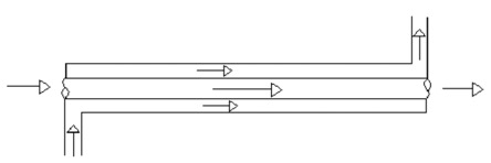
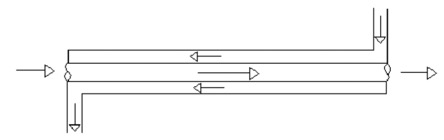
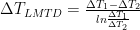
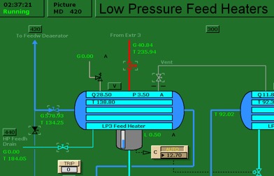
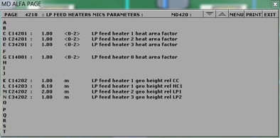
<div class="chapter standard" id="heat-exchangers"><div class="chapter-title-wrap"><h3 class="chapter-number">5</h3><h2 class="chapter-title">Heat Exchangers</h2></div><div class="ugc chapter-ugc"> <div class="bcc-box bcc-highlight"><h3>Learning Objectives</h3> <p>Operate the Plant in full generating capacity and study the effect of heat exchanger surface area using the Low Pressure Feed Heater 3.</p> </div> <h1>Theory</h1> <p>A heat exchanger is equipment in which heat exchange takes place between two working media that enter and exit at different temperatures. The main function of heat exchanger is to either remove heat from a hot working media or to add heat to the cold working media. Depending on direction of working media-fluid flow the heat exchanger is either parallel (concurrent) flow heat exchanger or counter flow heat exchanger (see Figures below).</p> <div id="attachment_91" style="max-width: 454px" class="wp-caption aligncenter"><a href="https://pressbooks.bccampus.ca/tpps/wp-content/uploads/sites/134/2017/03/Concurrent.jpg"><img src="https://pressbooks.bccampus.ca/tpps/wp-content/uploads/sites/134/2017/03/Concurrent.jpg" alt="Concurrent flow." class="size-full wp-image-91" width="444" height="148" srcset="https://pressbooks.bccampus.ca/tpps/wp-content/uploads/sites/134/2017/03/Concurrent.jpg 444w, https://pressbooks.bccampus.ca/tpps/wp-content/uploads/sites/134/2017/03/Concurrent-300x100.jpg 300w, https://pressbooks.bccampus.ca/tpps/wp-content/uploads/sites/134/2017/03/Concurrent-65x22.jpg 65w, https://pressbooks.bccampus.ca/tpps/wp-content/uploads/sites/134/2017/03/Concurrent-225x75.jpg 225w, https://pressbooks.bccampus.ca/tpps/wp-content/uploads/sites/134/2017/03/Concurrent-350x117.jpg 350w" /></a> <p class="wp-caption-text">Concurrent flow.</p> </div> <div id="attachment_90" style="max-width: 454px" class="wp-caption aligncenter"><a href="https://pressbooks.bccampus.ca/tpps/wp-content/uploads/sites/134/2017/03/Counter.jpg"><img src="https://pressbooks.bccampus.ca/tpps/wp-content/uploads/sites/134/2017/03/Counter.jpg" alt="Counter current flow." class="size-full wp-image-90" width="444" height="140" srcset="https://pressbooks.bccampus.ca/tpps/wp-content/uploads/sites/134/2017/03/Counter.jpg 444w, https://pressbooks.bccampus.ca/tpps/wp-content/uploads/sites/134/2017/03/Counter-300x95.jpg 300w, https://pressbooks.bccampus.ca/tpps/wp-content/uploads/sites/134/2017/03/Counter-65x20.jpg 65w, https://pressbooks.bccampus.ca/tpps/wp-content/uploads/sites/134/2017/03/Counter-225x71.jpg 225w, https://pressbooks.bccampus.ca/tpps/wp-content/uploads/sites/134/2017/03/Counter-350x110.jpg 350w" /></a> <p class="wp-caption-text">Counter current flow.</p> </div> <p>The terms are related to how the fluid flows through their respective flow passages relative to each other. If fluids flow in the same direction such as in Figure 1 it is termed a parallel flow. If fluids flow in opposite directions as in Figure 2 it is termed counter flow.</p> <p>Parallel flow in heat exchangers occurs when both fluids enter the heat exchanger at their largest temperature difference. The temperature difference becomes less over the length of the heat exchanger. In the counter flow heat exchanger, fluids enter at opposite ends and therefore at different ends of the temperature scale Figure 2. The temperature difference between two fluids is relatively constant over the length of the exchanger.</p> <p>The heat transfer process that occurs in any heat exchanger can be described by the following equations.</p> <p style="text-align: center"><img src="https://s0.wp.com/latex.php?latex=Q_%7Bhot%7D+%3D+m_%7Bhot%7Dc_%7Bp+hot%7D%5CDelta+T_%7Bhot%7D&#38;bg=T&#38;fg=000000&#38;s=0&#38;zoom=1" alt="Q_{hot} = m_{hot}c_{p hot}\Delta T_{hot}" title="Q_{hot} = m_{hot}c_{p hot}\Delta T_{hot}" class="latex" /><br /> <img src="https://s0.wp.com/latex.php?latex=Q_%7Bcold%7D+%3D+m_%7Bcold%7Dc_%7Bp+cold%7D%5CDelta+T_%7Bcold%7D&#38;bg=T&#38;fg=000000&#38;s=0&#38;zoom=1" alt="Q_{cold} = m_{cold}c_{p cold}\Delta T_{cold}" title="Q_{cold} = m_{cold}c_{p cold}\Delta T_{cold}" class="latex" /></p> <p>Considering the surface area involved in heat transfer, Newton’s Law of cooling states that the rate of heat loss is proportional to the difference in temperatures between the body and its surroundings and given by,</p> <p style="text-align: center"><img src="https://s0.wp.com/latex.php?latex=Q+%3D+%5Calpha+Area+%5CDelta+T&#38;bg=T&#38;fg=000000&#38;s=0&#38;zoom=1" alt="Q = \alpha Area \Delta T" title="Q = \alpha Area \Delta T" class="latex" /></p> <p>where α is called the heat transfer coefficient [W/m<sup>2</sup>K], area is taken in m<sup>2</sup> and ΔT is the temperature difference.</p> <p>Furthermore Q, heat transferred between the hot water and cold water can be calculated as follows:</p> <p style="text-align: center"><img src="https://s0.wp.com/latex.php?latex=Q+%3D+%5Cfrac%7BF%28LMTD%29%7D%7BR_%7BT%7D%7D&#38;bg=T&#38;fg=000000&#38;s=0&#38;zoom=1" alt="Q = \frac{F(LMTD)}{R_{T}}" title="Q = \frac{F(LMTD)}{R_{T}}" class="latex" /></p> <p>Or</p> <p style="text-align: center"><img src="https://s0.wp.com/latex.php?latex=Q+%3D+F%28UA%29%28LMTD%29&#38;bg=T&#38;fg=000000&#38;s=0&#38;zoom=1" alt="Q = F(UA)(LMTD)" title="Q = F(UA)(LMTD)" class="latex" /></p> <p>where F is the correction factor which equals 1 for this SIMLAB (it takes values between 0.5 and 1). R<sub>T</sub> is the overall resistance, U, overall heat transfer coefficient and LMTD is the Log Mean Temperature Difference.</p> <p>The overall resistances can be calculated using:</p> <p style="text-align: center"><img src="https://s0.wp.com/latex.php?latex=R_%7BT%7D%3DR_%7Bhf%7D%2BR_%7Bw%7D%2BR_%7Bcf%7D&#38;bg=T&#38;fg=000000&#38;s=0&#38;zoom=1" alt="R_{T}=R_{hf}+R_{w}+R_{cf}" title="R_{T}=R_{hf}+R_{w}+R_{cf}" class="latex" /></p> <p style="text-align: center"><img src="https://s0.wp.com/latex.php?latex=R_%7Bhf%7D+%3D+%5Cfrac%7B1%7D%7BA_%7B1%7D%5Calpha_%7Bh%7D%7D&#38;bg=T&#38;fg=000000&#38;s=0&#38;zoom=1" alt="R_{hf} = \frac{1}{A_{1}\alpha_{h}}" title="R_{hf} = \frac{1}{A_{1}\alpha_{h}}" class="latex" /></p> <p style="text-align: center"><img src="https://s0.wp.com/latex.php?latex=R_%7Bw%7D+%3D+%5Cfrac%7Bln%5Cfrac%7BD_%7B2%7D%7D%7BD_%7B1%7D%7D%7D%7B2%5Cpi+L%5Clambda_%7Bw%7D%7D&#38;bg=T&#38;fg=000000&#38;s=0&#38;zoom=1" alt="R_{w} = \frac{ln\frac{D_{2}}{D_{1}}}{2\pi L\lambda_{w}}" title="R_{w} = \frac{ln\frac{D_{2}}{D_{1}}}{2\pi L\lambda_{w}}" class="latex" /></p> <p style="text-align: center"><img src="https://s0.wp.com/latex.php?latex=R_%7Bcf%7D+%3D+%5Cfrac%7B1%7D%7BA_%7B2%7D%5Calpha_%7Bc%7D%7D&#38;bg=T&#38;fg=000000&#38;s=0&#38;zoom=1" alt="R_{cf} = \frac{1}{A_{2}\alpha_{c}}" title="R_{cf} = \frac{1}{A_{2}\alpha_{c}}" class="latex" /></p> <p>Heat transfer coefficients ah and ac can be calculated using the following expression for Nusselt number for hot and cold water:</p> <p>For cooling</p> <p style="text-align: center"><img src="https://s0.wp.com/latex.php?latex=%5Calpha_%7Bh%7D+%3D+%5Cfrac%7BNu_%7Bh%7D%5Clambda_%7Bh%7D%7D%7BD_%7Bh%7D%7D&#38;bg=T&#38;fg=000000&#38;s=0&#38;zoom=1" alt="\alpha_{h} = \frac{Nu_{h}\lambda_{h}}{D_{h}}" title="\alpha_{h} = \frac{Nu_{h}\lambda_{h}}{D_{h}}" class="latex" /></p> <p style="text-align: center"><img src="https://s0.wp.com/latex.php?latex=Nu_%7Bh%7D+%3D+0.3Re_%7Bh%7D%5E%7B0.8%7DPr_%7Bh%7D%5E%7B0.3%7D&#38;bg=T&#38;fg=000000&#38;s=0&#38;zoom=1" alt="Nu_{h} = 0.3Re_{h}^{0.8}Pr_{h}^{0.3}" title="Nu_{h} = 0.3Re_{h}^{0.8}Pr_{h}^{0.3}" class="latex" /></p> <p>&nbsp;</p> <p>For heating</p> <p style="text-align: center"><img src="https://s0.wp.com/latex.php?latex=%5Calpha_%7Bc%7D+%3D+%5Cfrac%7BNu_%7Bc%7D%5Clambda_%7Bc%7D%7D%7BD_%7Bc%7D%7D&#38;bg=T&#38;fg=000000&#38;s=0&#38;zoom=1" alt="\alpha_{c} = \frac{Nu_{c}\lambda_{c}}{D_{c}}" title="\alpha_{c} = \frac{Nu_{c}\lambda_{c}}{D_{c}}" class="latex" /></p> <p style="text-align: center"><img src="https://s0.wp.com/latex.php?latex=Nu_%7Bc%7D+%3D+0.3Re_%7Bc%7D%5E%7B0.8%7DPr_%7Bc%7D%5E%7B0.3%7D&#38;bg=T&#38;fg=000000&#38;s=0&#38;zoom=1" alt="Nu_{c} = 0.3Re_{c}^{0.8}Pr_{c}^{0.3}" title="Nu_{c} = 0.3Re_{c}^{0.8}Pr_{c}^{0.3}" class="latex" /></p> <p>And the LMTD is given by the following correlation where 1 and 2 presents the ends of the heat exchanger:</p> <p style="text-align: center"><img src="https://s0.wp.com/latex.php?latex=%5CDelta+T_%7BLMTD%7D+%3D+%5Cfrac%7B%5CDelta+T_%7B1%7D-%5CDelta+T_%7B2%7D%7D%7Bln%5Cfrac%7B%5CDelta+T_%7B1%7D%7D%7B%5CDelta+T_%7B2%7D%7D%7D&#38;bg=T&#38;fg=000000&#38;s=0&#38;zoom=1" alt="\Delta T_{LMTD} = \frac{\Delta T_{1}-\Delta T_{2}}{ln\frac{\Delta T_{1}}{\Delta T_{2}}}" title="\Delta T_{LMTD} = \frac{\Delta T_{1}-\Delta T_{2}}{ln\frac{\Delta T_{1}}{\Delta T_{2}}}" class="latex" /></p> <h2>Heat Exchanger Effectiveness</h2> <p>Recall from the <a href="https://pressbooks.bccampus.ca/tpps/chapter/boiler-efficiency/">Boiler Efficiency</a> Lab that <span itemscope="itemscope" itemtype="http://schema.org/WebPage">efficiency is to do with minimizing waste and effectiveness to do with maximizing output. Here we define</span> heat exchanger effectiveness as the ratio of actual heat transfer rate to the maximum possible heat transfer rate for the given temperatures.</p> <p style="text-align: center"><img src="https://s0.wp.com/latex.php?latex=%5Cepsilon+%3D+%5Cfrac%7BQ%7D%7BQ_%7Bmax%7D%7D&#38;bg=T&#38;fg=000000&#38;s=0&#38;zoom=1" alt="\epsilon = \frac{Q}{Q_{max}}" title="\epsilon = \frac{Q}{Q_{max}}" class="latex" /></p> <p style="text-align: center"><img src="https://s0.wp.com/latex.php?latex=Q_%7Bmax%7D+%3D+C_%7Bmin%7D%28T_%7Bhi%7D-T_%7Bci%7D%29&#38;bg=T&#38;fg=000000&#38;s=0&#38;zoom=1" alt="Q_{max} = C_{min}(T_{hi}-T_{ci})" title="Q_{max} = C_{min}(T_{hi}-T_{ci})" class="latex" /></p> <p>Where C<sub>min</sub> is defined either by cold or hot fluid whichever is smaller and it is defined by:</p> <p style="text-align: center"><img src="https://s0.wp.com/latex.php?latex=C_%7Bh%7D+%3D+m_%7Bh%7Dc_%7Bph%7D&#38;bg=T&#38;fg=000000&#38;s=0&#38;zoom=1" alt="C_{h} = m_{h}c_{ph}" title="C_{h} = m_{h}c_{ph}" class="latex" /></p> <p style="text-align: center"><img src="https://s0.wp.com/latex.php?latex=C_%7Bc%7D+%3D+m_%7Bc%7Dc_%7Bpc%7D&#38;bg=T&#38;fg=000000&#38;s=0&#38;zoom=1" alt="C_{c} = m_{c}c_{pc}" title="C_{c} = m_{c}c_{pc}" class="latex" /></p> <p>&nbsp;</p> <div class="textbox learning-objectives"><h3>Lab Instructions</h3> <p>Run the initial condition I10 230 MW_oil_auto and setup trends for</p> <div style="margin: auto;"><table><tbody><tr><td>Heat Area Factor</td> <td>C34201</td> </tr> <tr><td>Q</td> <td>Q34228</td> </tr> <tr><td>T<sub>cold1</sub></td> <td>T24214</td> </tr> <tr><td>T<sub>cold2</sub></td> <td>T34214</td> </tr> <tr><td>m<sub>cold</sub></td> <td>G34213</td> </tr> <tr><td>T<sub>hot1</sub></td> <td>T34204</td> </tr> <tr><td>T<sub>hot2</sub></td> <td>T34227</td> </tr> <tr><td>m<sub>hot</sub></td> <td>G34203</td> </tr> </tbody> </table> </div> <ol><li><strong>Heat Area Factor set to 0.5: </strong>Using MD420 and Variable List 4210 set C34201 to 0.5. Run the simulator with this setting for 15 minutes. Freeze and print the two trends.</li> <li><strong>Heat Area Factor set to 1:</strong> As in step 1, set C34201 to 1. This is the default setting for the Heat Area Factor (heat transfer coefficient x area). After 15 minutes of running the simulator, freeze simulator and print the two trends.</li> <li><strong>Heat Area Factor set to 1.5: </strong>This time, set C34201 to 1.5. Run the simulator with this setting for 15 minutes. Freeze and print the two trends.</li> </ol> </div> <h2 style="text-align: left">Hints &amp; Tips</h2> <p>As always, label your trends using descriptive names. In this lab, you are changing the Heat Area Factor (heat transfer coefficient x area) of LP Feed Heater 3 and comparing the temperature data. Your evaluation will be based on LMTD and Heat Exchanger Effectiveness values.</p> <div id="attachment_89" style="max-width: 402px" class="wp-caption aligncenter"><a href="https://pressbooks.bccampus.ca/tpps/wp-content/uploads/sites/134/2017/03/MD420.jpg"><img src="https://pressbooks.bccampus.ca/tpps/wp-content/uploads/sites/134/2017/03/MD420.jpg" alt="MD420 LP Feed Heater 3" class="size-full wp-image-89" width="392" height="252" srcset="https://pressbooks.bccampus.ca/tpps/wp-content/uploads/sites/134/2017/03/MD420.jpg 392w, https://pressbooks.bccampus.ca/tpps/wp-content/uploads/sites/134/2017/03/MD420-300x193.jpg 300w, https://pressbooks.bccampus.ca/tpps/wp-content/uploads/sites/134/2017/03/MD420-65x42.jpg 65w, https://pressbooks.bccampus.ca/tpps/wp-content/uploads/sites/134/2017/03/MD420-225x145.jpg 225w, https://pressbooks.bccampus.ca/tpps/wp-content/uploads/sites/134/2017/03/MD420-350x225.jpg 350w" /></a> <p class="wp-caption-text">MD420 LP Feed Heater 3</p> </div> <div id="attachment_88" style="max-width: 404px" class="wp-caption aligncenter"><a href="https://pressbooks.bccampus.ca/tpps/wp-content/uploads/sites/134/2017/03/VariableList4210.jpg"><img src="https://pressbooks.bccampus.ca/tpps/wp-content/uploads/sites/134/2017/03/VariableList4210.jpg" alt="Variable List 4210." class="size-full wp-image-88" width="394" height="195" srcset="https://pressbooks.bccampus.ca/tpps/wp-content/uploads/sites/134/2017/03/VariableList4210.jpg 394w, https://pressbooks.bccampus.ca/tpps/wp-content/uploads/sites/134/2017/03/VariableList4210-300x148.jpg 300w, https://pressbooks.bccampus.ca/tpps/wp-content/uploads/sites/134/2017/03/VariableList4210-65x32.jpg 65w, https://pressbooks.bccampus.ca/tpps/wp-content/uploads/sites/134/2017/03/VariableList4210-225x111.jpg 225w, https://pressbooks.bccampus.ca/tpps/wp-content/uploads/sites/134/2017/03/VariableList4210-350x173.jpg 350w" /></a> <p class="wp-caption-text">Variable List 4210.</p> </div> <div class="textbox learning-objectives"><h3>Deliverables</h3> <p>Your lab report is to include the following:</p> <ul><li><strong>Trend plots:</strong> Supply all plots taken for this lab, make sure they are labelled properly.</li> <li><strong>Computation:</strong> Use MATLAB or MS Excel and calculate the LMTD and Heat Exchanger effectiveness values for the 3 tests.</li> <li><strong>Conclusion:</strong> Write a summary (max. 500 words, in a text box if using Excel) comparing your results and suggestions for further study.</li> </ul> </div> <div class="textbox shaded"><p>Further Reading:</p> <ul><li>Applied Thermodynamics for Engineering Technologists by T. D. Eastop and A. McConkey: Heat Transfer.</li> </ul> </div> </div>
</div>
<div class="chapter standard" id="combustion-analysis"><div class="chapter-title-wrap"><h3 class="chapter-number">6</h3><h2 class="chapter-title">Combustion Analysis</h2></div><div class="ugc chapter-ugc"> <div class="bcc-box bcc-highlight"><h3>Learning Objectives</h3> <p>Operate the Plant at 80% capacity burning coal to</p> <ul><li>Perform combustion analyses for two types of coal,</li> <li>Compare results.</li> </ul> </div> <h1>Theory</h1> <p>In the <a href="https://pressbooks.bccampus.ca/tpps/chapter/boiler-efficiency/" target="_blank">Boiler Efficiency</a> lab, we stated that Combustion Efficiency is defined as the ratio of the burner’s capability to burn fuel completely to the unburned fuel and excess air in the exhaust. In this lab, we will perform a combustion analysis.</p> <p>Fossil fuels may be classified into solid, liquid and gaseous fuels. The vast majority of fuels are based on carbon (C), hydrogen (H<sub>2</sub>) or some combination of carbon and hydrogen called hydrocarbons.</p> <p>During combustion, oxygen (O<sub>2</sub>) combines rapidly with C, H<sub>2</sub>, sulphur (S<sub>2</sub>) and their compounds in solid, liquid and gaseous fuels and results in the liberation of energy. Except for special applications such as oxyacetylene welding, in which a high-temperature flame is required, the O<sub>2 </sub>necessary for combustion is obtained from air. Air contains O<sub>2</sub> and nitrogen (N<sub>2</sub>), plus negligible amounts of other gasses and for engineering purposes, may be considered to have the following percentage composition by mass:</p> <p style="text-align: center">O<sub>2</sub>: 23%<br /> N<sub>2</sub>: 77%</p> <p>The proportions in which the elements enter into the combustion reaction by mass are dependent upon the relative molecular weights as shown below:</p> <table style="width: 370.267px"><tbody><tr><td style="width: 112px"><strong>Element</strong></td> <td style="width: 112px"><strong>Symbol</strong></td> <td style="width: 112px"><strong>Molecular Weight</strong></td> </tr> <tr><td style="width: 112px">Carbon</td> <td style="width: 112px">C</td> <td style="width: 112.267px">12</td> </tr> <tr><td style="width: 112px">Sulphur</td> <td style="width: 112px">S<sub>2</sub></td> <td style="width: 112.267px">32</td> </tr> <tr><td style="width: 112px">Hydrogen</td> <td style="width: 112px">H<sub>2</sub></td> <td style="width: 112.267px">2</td> </tr> <tr><td style="width: 112px">Oxygen</td> <td style="width: 112px">O<sub>2</sub></td> <td style="width: 112.267px">32</td> </tr> <tr><td style="width: 112px">Nitrogen</td> <td style="width: 112px">N<sub>2</sub></td> <td style="width: 112.267px">28</td> </tr> </tbody> </table> <h1>Stoichiometric Combustion Theory</h1> <p>Complete combustion of simple hydrocarbon fuels forms carbon dioxide (C0<sub>2</sub>) from the carbon and water (H<sub>2</sub>0) from the hydrogen, so for a hydrocarbon fuel with the general composition C<sub>n</sub>H<sub>m</sub>, the combustion equation on a molar basis is as flows:</p> <p style="text-align: center"><img src="https://s0.wp.com/latex.php?latex=C_%7Bn%7DH_%7Bm%7D%2ByO_%7B2%7D%5Crightarrow+aCO_%7B2%7D%2BbH_%7B2%7DO&#38;bg=T&#38;fg=000000&#38;s=0&#38;zoom=1" alt="C_{n}H_{m}+yO_{2}\rightarrow aCO_{2}+bH_{2}O" title="C_{n}H_{m}+yO_{2}\rightarrow aCO_{2}+bH_{2}O" class="latex" /></p> <p>Where the balance should be satisfied following the moles for any mathematcial  equation:</p> <p>Carbon balance:</p> <p style="text-align: center"><img src="https://s0.wp.com/latex.php?latex=a%3Dn&#38;bg=T&#38;fg=000000&#38;s=0&#38;zoom=1" alt="a=n" title="a=n" class="latex" /> kmol CO<sub>2</sub>/ kmol fuel</p> <p style="text-align: left">Hydrogen balance:</p> <p style="text-align: center"><img src="https://s0.wp.com/latex.php?latex=2b%3Dm&#38;bg=T&#38;fg=000000&#38;s=0&#38;zoom=1" alt="2b=m" title="2b=m" class="latex" /> </p> <p style="text-align: center"><img src="https://s0.wp.com/latex.php?latex=b+%3D+%5Cfrac%7Bm%7D%7B2%7D&#38;bg=T&#38;fg=000000&#38;s=0&#38;zoom=1" alt="b = \frac{m}{2}" title="b = \frac{m}{2}" class="latex" /> kmol H<sub>2</sub>O/ kmol fuel</p> <p>Oxygen balance:</p> <p style="text-align: center"><img src="https://s0.wp.com/latex.php?latex=2y+%3D+2a%2Bb&#38;bg=T&#38;fg=000000&#38;s=0&#38;zoom=1" alt="2y = 2a+b" title="2y = 2a+b" class="latex" /></p> <p style="text-align: center"><img src="https://s0.wp.com/latex.php?latex=y+%3D+a%2B%5Cfrac%7Bb%7D%7B2%7D&#38;bg=T&#38;fg=000000&#38;s=0&#38;zoom=1" alt="y = a+\frac{b}{2}" title="y = a+\frac{b}{2}" class="latex" /> kmol O<sub>2</sub>/ kmol fuel </p> <p>Considering that combustion occurs in air rather than in pure oxygen, the nitrogen in the air may react in the combustion process to produce nitrogen oxides. Beside, some fuels contain elements other than carbon, and these elements may react with oxygen during combustion. Also, combustion is not always complete, and the exhaust gases contain unburned and partially burned products in addition to C0<sub>2</sub> and H<sub>2</sub>O.</p> <p>Air is composed of oxygen, nitrogen, and small amounts of carbon dioxide, argon, and other trace components. For the purposes of the further calculation it is perfectly reasonable to consider air as a mixture of 21% (mole basis) 02 and 79 % (mole basis) N<sub>2</sub>.  Nitrogen will be considered as an “inert&#8221; gas in the combustion calculations. The stoichiometric relation for complete combustion of a hydrocarbon fuel, C<sub>n</sub>H<sub>m</sub>, becomes</p> <p style="text-align: center"><img src="https://s0.wp.com/latex.php?latex=C_%7Bn%7DH_%7Bm%7D%2By%28O_%7B2%7D%2B%5Cfrac%7B79%7D%7B21%7DN_%7B2%7D%5Crightarrow+aCO_%7B2%7D%2BbH_%7B2%7DO%2BcN_%7B2%7D&#38;bg=T&#38;fg=000000&#38;s=0&#38;zoom=1" alt="C_{n}H_{m}+y(O_{2}+\frac{79}{21}N_{2}\rightarrow aCO_{2}+bH_{2}O+cN_{2}" title="C_{n}H_{m}+y(O_{2}+\frac{79}{21}N_{2}\rightarrow aCO_{2}+bH_{2}O+cN_{2}" class="latex" /></p> <p>The balance equations are:</p> <p>Carbon balance:</p> <p style="text-align: center"><img src="https://s0.wp.com/latex.php?latex=a%3Dn&#38;bg=T&#38;fg=000000&#38;s=0&#38;zoom=1" alt="a=n" title="a=n" class="latex" /> kmol CO<sub>2</sub>/ kmol fuel</p> <p style="text-align: left">Hydrogen balance:</p> <p style="text-align: center"><img src="https://s0.wp.com/latex.php?latex=2b%3Dm&#38;bg=T&#38;fg=000000&#38;s=0&#38;zoom=1" alt="2b=m" title="2b=m" class="latex" /> </p> <p style="text-align: center"><img src="https://s0.wp.com/latex.php?latex=b+%3D+%5Cfrac%7Bm%7D%7B2%7D&#38;bg=T&#38;fg=000000&#38;s=0&#38;zoom=1" alt="b = \frac{m}{2}" title="b = \frac{m}{2}" class="latex" /> kmol H<sub>2</sub>O/ kmol fuel</p> <p>Oxygen balance:</p> <p style="text-align: center"><img src="https://s0.wp.com/latex.php?latex=2y+%3D+2a%2Bb&#38;bg=T&#38;fg=000000&#38;s=0&#38;zoom=1" alt="2y = 2a+b" title="2y = 2a+b" class="latex" /></p> <p style="text-align: center"><img src="https://s0.wp.com/latex.php?latex=y+%3D+a%2B%5Cfrac%7Bb%7D%7B2%7D&#38;bg=T&#38;fg=000000&#38;s=0&#38;zoom=1" alt="y = a+\frac{b}{2}" title="y = a+\frac{b}{2}" class="latex" /> kmol O<sub>2</sub>/ kmol fuel </p> <p>Nitrogen balance:</p> <p style="text-align: center"><img src="https://s0.wp.com/latex.php?latex=y%5Cfrac%7B79%7D%7B21%7D%3Dc&#38;bg=T&#38;fg=000000&#38;s=0&#38;zoom=1" alt="y\frac{79}{21}=c" title="y\frac{79}{21}=c" class="latex" /> kmol N<sub>2</sub>/kmol fuel</p> <p>Flue gas compositions are presented in terms of mole fractions as kmol of product per kmol of fuel.</p> <p>Example 1.  Combustion of Octane in Air</p> <p>Determine the stoichiometric air/ fuel mass ratio and product gas composition for combustion of octane ( C<sub>8</sub>H<sub>18</sub>)  in air.</p> <p style="text-align: center"><img src="https://s0.wp.com/latex.php?latex=C_%7B8%7DH_%7B18%7D%2By%28O_%7B2%7D%2B%5Cfrac%7B79%7D%7B21%7DN_%7B2%7D%5Crightarrow+aCO_%7B2%7D%2BbH_%7B2%7DO%2BcN_%7B2%7D&#38;bg=T&#38;fg=000000&#38;s=0&#38;zoom=1" alt="C_{8}H_{18}+y(O_{2}+\frac{79}{21}N_{2}\rightarrow aCO_{2}+bH_{2}O+cN_{2}" title="C_{8}H_{18}+y(O_{2}+\frac{79}{21}N_{2}\rightarrow aCO_{2}+bH_{2}O+cN_{2}" class="latex" /></p> <p>Carbon balance:</p> <p style="text-align: center"><img src="https://s0.wp.com/latex.php?latex=a%3Dn%3D8&#38;bg=T&#38;fg=000000&#38;s=0&#38;zoom=1" alt="a=n=8" title="a=n=8" class="latex" /> kmol CO<sub>2</sub>/ kmol fuel</p> <p style="text-align: left">Hydrogen balance:</p> <p style="text-align: center"><img src="https://s0.wp.com/latex.php?latex=2b%3D18&#38;bg=T&#38;fg=000000&#38;s=0&#38;zoom=1" alt="2b=18" title="2b=18" class="latex" /> </p> <p style="text-align: center"><img src="https://s0.wp.com/latex.php?latex=b+%3D+%5Cfrac%7B18%7D%7B2%7D%3D9&#38;bg=T&#38;fg=000000&#38;s=0&#38;zoom=1" alt="b = \frac{18}{2}=9" title="b = \frac{18}{2}=9" class="latex" /> kmol H<sub>2</sub>O/ kmol fuel</p> <p>Oxygen balance:</p> <p style="text-align: center"><img src="https://s0.wp.com/latex.php?latex=2y+%3D+2%288%29%2Bb&#38;bg=T&#38;fg=000000&#38;s=0&#38;zoom=1" alt="2y = 2(8)+b" title="2y = 2(8)+b" class="latex" /></p> <p style="text-align: center"><img src="https://s0.wp.com/latex.php?latex=y+%3D+8%2B%5Cfrac%7B9%7D%7B2%7D%3D12.5&#38;bg=T&#38;fg=000000&#38;s=0&#38;zoom=1" alt="y = 8+\frac{9}{2}=12.5" title="y = 8+\frac{9}{2}=12.5" class="latex" /> kmol O<sub>2</sub>/ kmol fuel </p> <p>Nitrogen balance:</p> <p style="text-align: center"><img src="https://s0.wp.com/latex.php?latex=y%5Cfrac%7B79%7D%7B21%7D%3Dc%3D12.5%5Cfrac%7B79%7D%7B21%7D%3D47&#38;bg=T&#38;fg=000000&#38;s=0&#38;zoom=1" alt="y\frac{79}{21}=c=12.5\frac{79}{21}=47" title="y\frac{79}{21}=c=12.5\frac{79}{21}=47" class="latex" /> kmol N<sub>2</sub>/kmol fuel</p> <p>The combustion equation becomes:</p> <p style="text-align: center"><img src="https://s0.wp.com/latex.php?latex=C_%7B8%7DH_%7B18%7D%2B12.5%28O_%7B2%7D%2B%5Cfrac%7B79%7D%7B21%7DN_%7B2%7D%5Crightarrow+8CO_%7B2%7D%2B9H_%7B2%7DO%2B47N_%7B2%7D&#38;bg=T&#38;fg=000000&#38;s=0&#38;zoom=1" alt="C_{8}H_{18}+12.5(O_{2}+\frac{79}{21}N_{2}\rightarrow 8CO_{2}+9H_{2}O+47N_{2}" title="C_{8}H_{18}+12.5(O_{2}+\frac{79}{21}N_{2}\rightarrow 8CO_{2}+9H_{2}O+47N_{2}" class="latex" /></p> <p style="text-align: left">Air/ fuel mass based ratio considering that 1 kmol fuel is 114 kg of fuel ( 8*12 + 18 *(1) = 114):</p> <p style="text-align: center"><img src="https://s0.wp.com/latex.php?latex=12.5%5Cfrac%7Bkmol%5C+O_%7B2%7D%7D%7Bkmol%5C+fuel%7D%5Cfrac%7B1%5C+kmol%5C+fuel%7D%7B114%5C+kg%5C+fuel%7D32%5Cfrac%7Bkg%5C+O_%7B2%7D%7D%7Bkmol%5C+O_%7B2%7D%7D%5Cfrac%7B100%5C+kg%5C+air%7D%7B23%5C+kg%5C+O_%7B2%7D%7D%3D15.25%5Cfrac%7Bkg%5C+air%7D%7Bkg%5C+fuel%7D&#38;bg=T&#38;fg=000000&#38;s=0&#38;zoom=1" alt="12.5\frac{kmol\ O_{2}}{kmol\ fuel}\frac{1\ kmol\ fuel}{114\ kg\ fuel}32\frac{kg\ O_{2}}{kmol\ O_{2}}\frac{100\ kg\ air}{23\ kg\ O_{2}}=15.25\frac{kg\ air}{kg\ fuel}" title="12.5\frac{kmol\ O_{2}}{kmol\ fuel}\frac{1\ kmol\ fuel}{114\ kg\ fuel}32\frac{kg\ O_{2}}{kmol\ O_{2}}\frac{100\ kg\ air}{23\ kg\ O_{2}}=15.25\frac{kg\ air}{kg\ fuel}" class="latex" /></p> <p style="text-align: left">Flue gas composition on molar basis is:</p> <p>Total number of kmol of flue gasses = kmol CO<sub>2</sub>  + kmol H<sub>2</sub>O + kmol N<sub>2</sub> = 8 +9+ 47 = 64 kmol flue gasses/ kmol fuel</p> <p>CO<sub>2</sub>  = 8/64 = 12.5 %</p> <p>H<sub>2</sub>O = 9/64 = 14 %</p> <p style="text-align: left">N<sub>2</sub> = 47/64 = 73.5%</p> <p>Other components and impurities in the fuel make the calculation process more complicated. For example if sulfur exists in fuel it is usually combust into sulfur dioxide (SO<sub>2</sub>). Ash, the noncombustible inorganic (mineral) impurities in the fuel, undergoes a number of transformations at combustion temperatures, will be neglected in the further calculation (ash will be assumed to be inert).</p> <p>For most solid and liquid fuels, the chemical composition is on a mass basis, as determined in the ultimate analysis.</p> <h2>Mass Based Chemistry of Combustion</h2> <p>The combustion reactions are written following the stoichiometric rules as defined above. The quantity of matter entering into a reaction is equal to the quantity of matter in the products of the reaction.</p> <p>The reaction for the complete combustion of C may be written as follows:</p> <p style="text-align: center">C+O<sub>2</sub>=CO<sub>2</sub></p> <p>or, if molecular weights are used,</p> <p style="text-align: center">12+32=44</p> <p style="text-align: center">1 kg C + 2⅔ kg O<sub>2</sub> = 3⅔ kg CO<sub>2</sub></p> <p>The complete combustion of H<sub>2</sub> occurs as follows:</p> <p style="text-align: center">2H<sub>2</sub> +O<sub>2</sub> =2H<sub>2</sub>O</p> <p style="text-align: center">4+32=36</p> <p style="text-align: center">1 kg H<sub>2</sub> + 8 kg O<sub>2</sub> = 9 kg H<sub>2</sub>O</p> <p style="text-align: left">Sulphur burns as follows:</p> <p style="text-align: center">S +O<sub>2</sub> =SO<sub>2</sub></p> <p style="text-align: center">32+32=64</p> <p style="text-align: center">1 kg S + 1 kg O<sub>2</sub> = 2 kg SO<sub>2</sub></p> <p>In addition, 1 kg of O<sub>2</sub> (<strong>stoichiometric mass of O<sub>2</sub></strong>) is contained in 1/0.232=4.3 kg air which is the <strong>stoichiometric mass of air</strong>. This air will contain 4.3-1=3.3 kg N<sub>2</sub>. Therefore we can write:</p> <p style="text-align: center">1 kg S + 4.3 kg air = 2 kg SO<sub>2</sub>+3.3 kg N<sub>2</sub></p> <h1 style="text-align: left">Procedure</h1> <p style="text-align: left">If the analysis of fuel is given by mass, follow the steps below:</p> <ol><li style="text-align: left"><strong>Total O<sub>2</sub> required:</strong> Determine the mass of O<sub>2</sub> required for each constituent and find the total mass of O<sub>2 </sub>(Subtract any O<sub>2</sub> which may be in the fuel)</li> <li style="text-align: left"><strong>Stoichiometric air: </strong>Stoichiometric mass of air = O<sub>2</sub> required/0.232</li> <li style="text-align: left"><strong>Total</strong> <strong>mass of combustion products:</strong> Determine the % mass of each combustion product. For example, given C content of 84.9%, CO<sub>2</sub>=84.9/100*2⅔=3.11% and find the total mass of combustion products.</li> <li style="text-align: left"><strong>Analysis of combustion products by mass: </strong>Suppose the total mass of combustion products in step 3 has been found as 12.09 kg/kg fuel, then CO<sub>2</sub>=3.11/12.09*100=25.74. This means that 25.74% of the flue gas is CO<sub>2</sub>. Repeat this calculation for each constituent.</li> </ol> <div class="textbox learning-objectives"><h3>Lab Instructions</h3> <p>Run the initial condition I14 80% Coal and setup trends for the following variables:</p> <p style="text-align: center">X00820 X00821 X00822 X00823 X00824 E23356</p> <p style="text-align: center">G02196 G02197 X32419 X02419 G00831 H00830</p> <ol><li><strong>Burning default coal:</strong> After 10 minutes of running the simulator, freeze simulator and print the two trends. This is the reference point for the next step.</li> <li><strong>Burning poor quality</strong> <strong>coal:</strong> Switch to run mode and access Variable List page 0111 on MD180. Set the new values as shown below. After 10 minutes, freeze simulator and print the two trends. <ul><li>X00820: 70.40</li> <li>X00821: 5.10</li> <li>X00822: 1.10</li> <li>X00823: 12.50</li> <li>X00824: 1.60</li> <li>X00825: 9.30</li> </ul> </li> <li><strong>Computation:</strong> Compute the following values for both types of fuels: <ul><li>Total O<sub>2</sub> required</li> <li>Stoichiometric air</li> <li>Total mass of combustion products</li> <li>Analysis of combustion products by mass [%]: CO<sub>2</sub>, H<sub>2</sub>O, SO<sub>2</sub>, N<sub>2</sub></li> </ul> </li> <li><strong>Comparison:</strong> Compare your findings based on the following data: <ul><li>Furnace outlet SO<sub>x</sub> flow</li> <li>Furnace outlet NO<sub>x</sub> flow</li> <li>CO content in flue gas</li> <li>Oxygen content in flue gas</li> <li>Theoretical combustion air</li> <li>Coal Heat Value</li> </ul> </li> </ol> </div> <h2 style="text-align: left">Hints &amp; Tips</h2> <p>In this lab, you are carrying out two combustion analyses. For data collection, set up your trends, a sample trend plot is shown below (Make sure your trend printouts are labeled properly otherwise, data analysis will be very confusing):</p> <div id="attachment_55" style="max-width: 668px" class="wp-caption aligncenter"><a href="https://pressbooks.bccampus.ca/tpps/wp-content/uploads/sites/134/2017/03/TrendGroupCoal.jpg"><img src="https://pressbooks.bccampus.ca/tpps/wp-content/uploads/sites/134/2017/03/TrendGroupCoal.jpg" alt="Sample data for coal" width="658" height="520" class="size-full wp-image-55" srcset="https://pressbooks.bccampus.ca/tpps/wp-content/uploads/sites/134/2017/03/TrendGroupCoal.jpg 658w, https://pressbooks.bccampus.ca/tpps/wp-content/uploads/sites/134/2017/03/TrendGroupCoal-300x237.jpg 300w, https://pressbooks.bccampus.ca/tpps/wp-content/uploads/sites/134/2017/03/TrendGroupCoal-65x51.jpg 65w, https://pressbooks.bccampus.ca/tpps/wp-content/uploads/sites/134/2017/03/TrendGroupCoal-225x178.jpg 225w, https://pressbooks.bccampus.ca/tpps/wp-content/uploads/sites/134/2017/03/TrendGroupCoal-350x277.jpg 350w" /></a> <p class="wp-caption-text">Sample data for coal</p> </div> <p>To change the fuel composition use the Variable List Page#: 0111 on MD180:</p> <div style="max-width: 721px" class="wp-caption aligncenter"><a href="https://pressbooks.bccampus.ca/tpps/wp-content/uploads/sites/134/2017/03/PoorQualityFuel.jpg"><img src="https://pressbooks.bccampus.ca/tpps/wp-content/uploads/sites/134/2017/03/PoorQualityFuel.jpg" alt="Chemical composition of coal" width="711" height="351" class="size-full wp-image-49" srcset="https://pressbooks.bccampus.ca/tpps/wp-content/uploads/sites/134/2017/03/PoorQualityFuel.jpg 711w, https://pressbooks.bccampus.ca/tpps/wp-content/uploads/sites/134/2017/03/PoorQualityFuel-300x148.jpg 300w, https://pressbooks.bccampus.ca/tpps/wp-content/uploads/sites/134/2017/03/PoorQualityFuel-65x32.jpg 65w, https://pressbooks.bccampus.ca/tpps/wp-content/uploads/sites/134/2017/03/PoorQualityFuel-225x111.jpg 225w, https://pressbooks.bccampus.ca/tpps/wp-content/uploads/sites/134/2017/03/PoorQualityFuel-350x173.jpg 350w" /></a> <p class="wp-caption-text">Chemical composition of coal</p> </div> <div class="textbox learning-objectives"><h3>Deliverables</h3> <p>Your lab report is to include the following:</p> <ul><li><strong>Trend plots:</strong> Supply all plots taken for each of the 2 fuels,</li> <li><strong>Computation:</strong> As per lab instructions above, perform combustion analyses using MATLAB or MS Excel.</li> <li><strong>Conclusion:</strong> Write a summary (max. 500 words<span itemscope="itemscope" itemtype="http://schema.org/WebPage">, in a text box if using Excel</span>) comparing your results and suggestions for further study.</li> </ul> </div> <div class="textbox shaded"><p>Further Reading:</p> <ul><li>Basic Engineering Thermodynamics in SI Units by R. Joel: Combustion.</li> <li>Thermal Engineering by H.L. Solberg, O.C. Cromer and A.R. Spalding: Fossil fuels and their combustion.</li> <li><p id="firstHeading" class="firstHeading" xml:lang="en"><a href="https://en.wikipedia.org/wiki/Stoichiometry" target="_blank">Stoichiometry. </a></p> </li> </ul> </div> </div>
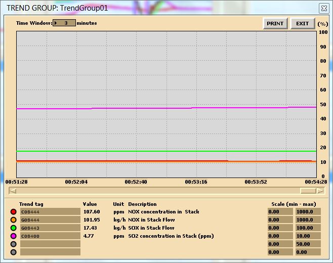
</div>
<div class="back-matter about-the-author" id="authors"><div class="back-matter-title-wrap"><h3 class="back-matter-number">1</h3><h1 class="back-matter-title">Authors</h1></div><div class="ugc back-matter-ugc"><p><strong>Sanja Boskovic</strong> is the Chief Instructor at the Power Engineering Group of <a href="https://www.bcit.ca/">BCIT</a> where she teaches Thermodynamics, Heat Transfer and Fluid Mechanics within the full time programs. Additionally, Sanja is the lead Thermodynamics and Applied Mechanics virtual classroom instructor for distance education and industry services courses. She was the 2011 recipient of BCIT Alumni Association Excellence in Teaching Award as well as the 2016 BCIT Teaching Excellence Award. Sanja is a member of the <a href="http://www.nipe.ca/index2.html" target="_blank" rel="noopener">Institute of Power Engineers</a> and <a href="https://www.asme.org/" target="_blank" rel="noopener">American Society of Mechanical Engineers</a>, and serves as a chair at <a href="http://www.ipecc-net.com/" target="_blank" rel="noopener">Interprovincial Power Engineering Curriculum Committee</a> and co-chair at Boiler Technology Committee at <a href="https://www.technicalsafetybc.ca/" target="_blank" rel="noopener">Technical Safety BC</a>. Sanja holds a PhD in Mechanical Engineering and a PhD in Educational Technology and Learning Design.</p> <p>&nbsp;</p> <p><strong>Serhat Beyenir</strong> is an instructor at the Power Engineering Group of <a href="https://www.bcit.ca/">BCIT</a> where he maintains web-based online courses and tutor distance education learners. He also teaches in the Power and Process Engineering program. Serhat is an open source software (OSS) advocate and open textbook proponent: He began to use OSS in 2001. Since then he has promoted Linux-variant operating systems, built content and learning management systems using Joomla, Drupal, WordPress and Moodle, and gave OSS related presentations. As a graduate student at Athabasca University, Serhat spent considerable time learning about open textbooks in his coursework and research assignments. Receiving a Master of Education degree in 2011, Serhat authored an <a href="http://opentextbook.docsol.sfu.ca/store/?product=OTB102-01" target="_blank" rel="noopener">open textbook</a> utilizing the Connexions platform and he has been distributing his book free of charge to Power Engineering students since October 2011.</p> </div>
</div>
<div class="back-matter miscellaneous" id="revision-history"><div class="back-matter-title-wrap"><h3 class="back-matter-number">2</h3><h1 class="back-matter-title">Revision History</h1></div><div class="ugc back-matter-ugc"><p>Version 0.7 – December 6, 2017 (Additional copy editing and proof reading)<br /> Version 0.6 – September 22, 2017 (Guest-lecturing at Kalmar Maritime Academy, Sweden)<br /> Version 0.5 – March 28, 2017 (BCIT OpenEd Week presentation)<br /> Version 0.4 – March 1, 2017 (Second Sprint event with our students)<br /> Version 0.3 – February 1, 2017 (First Sprint event with our students)<br /> Version 0.2 – December 19, 2016 (First draft)<br /> Version 0.1 – November 3, 2016 (Initial development)</p> </div>
</div>
</body>
</html>