Empirical Rule

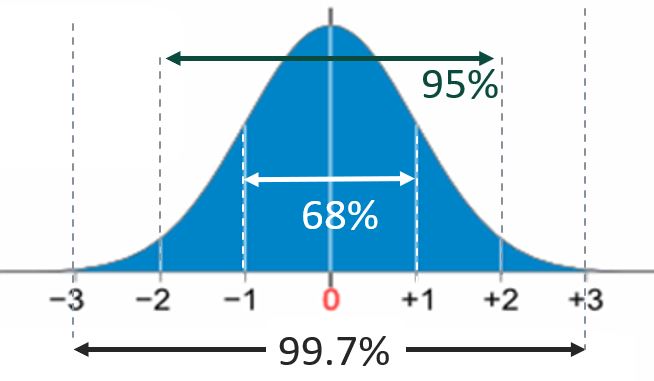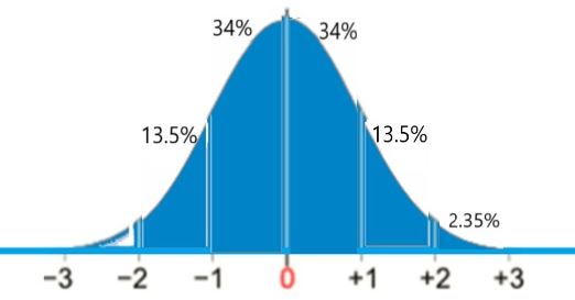
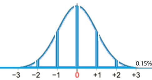
When data are Normally Distributed: Roughly 68% of all data are within 1 standard deviation of the mean Roughly 95% of all data are within 2 standard deviations of the mean Roughly 99.7% of all data are within 3 standard deviations of the mean

Outliers

Data beyond 3 standard deviations are called ‘outliers‘ Roughly 0.15% of the data are 3 standard deviations above or below the mean

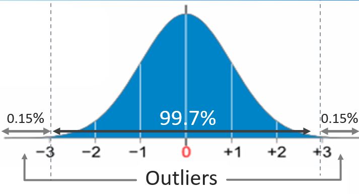Applying the Empirical Rule (Exercises)

Let us first try some examples/exercises where we will seek to understand the Empirical Rule percentages. This understanding will also help when calculating more complicated probabilities using Excel’s NORM.DIST() function in later sections.

Example 39.1

Problem Setup: In this problem, we will ‘divide up’ the sections of the normal curve into ‘slices’.

Question: Can you figure out the percent of data that lie in each slice of the curve?

You try: Drag the appropriate percentage into each slice in the exercise below:

Need Help? Try the exercise below first.

Example 39.2

Problem Setup: Demand for the 12-pack of extra plush toilet paper follows a normal distribution at a local drug store. On average, they sell 50 packs per week with a standard deviation of 10 packs. They get deliveries once per week and stock 80 packs of toilet paper per week.

Question: Can you solve for the probabilities below and match them to their answers?

Need Help? Click on the problems below to reveal their answers:

Probability of 40 to 60 packs sold

We are given the following values in the problem:

• μ = 50, σ = 10, x₁ = 40, x₂ = 60
• z₁ = ^(40−50)/₁₀ = ⁻¹⁰/₁₀ = −1
• z₂ = ^(60−50)/₁₀ = ¹⁰/₁₀ = 1

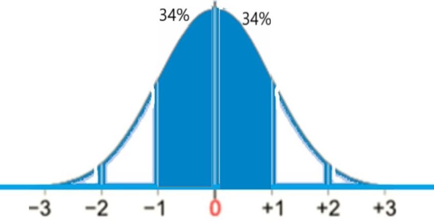
This gives P(40 < x < 60) = 34% + 34% = 68% (see below):

probability of 30 and 70 packs sold

We are given the following values in the problem:

• μ = 50, σ = 10, x₁ = 30, x₂ = 70
• z₁ = ^(30−50)/₁₀ = ⁻²⁰/₁₀ = −2
• z₂ = ^(70−50)/₁₀ = ²⁰/₁₀ = 2

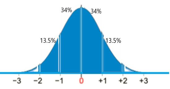
This gives P(30 < x < 70) = 13.5% + 34% + 34% + 13.5% = 95% (see below):

probability of 30 and 80 packs sold

We are given the following values in the problem:

• μ = 50, σ = 10, x₁ = 30, x₂ = 80
• z₁ = ^(30−50)/₁₀ = ⁻²⁰/₁₀ = −2
• z₂ = ^(80−50)/₁₀ = ³⁰/₁₀ = 3

This gives P(30 < x < 80) = 13.5% + 34% + 34% + 13.5% + 2.35% = 97.35% (see below):

probability of Less than 20 packs sold

We are given the following values in the problem:

• μ = 50, σ = 10, x = 20
• z = ^(20−50)/₁₀ = ⁻³⁰/₁₀ = −3

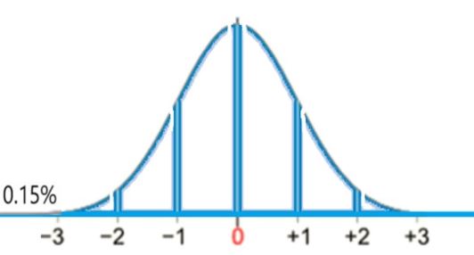
This gives P(x < 20) = 0.15% (see below):

probability of Greater than 50 packs sold

We are given the following values in the problem:

• μ = 50, σ = 10, x₁ = 30, x = 50
• z = ^(50−50)/₁₀ = ⁰/₁₀ = 0

This gives P(x > 50) = 34% + 13.5% + 0.15% = 50% (see below):

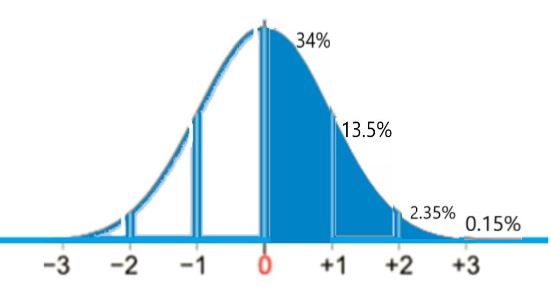
Conclusion: We see that the area above the mean (z=0) makes up half (50%) of the graph.

probability of 40 and 70 packs sold

We are given the following values in the problem:

• μ = 50, σ = 10, x₁ = 40, x₂ = 70
• z₁ = ^(40−50)/₁₀ = ⁻¹⁰/₁₀ = −1
• z₂ = ^(70−50)/₁₀ = ²⁰/₁₀ = 2

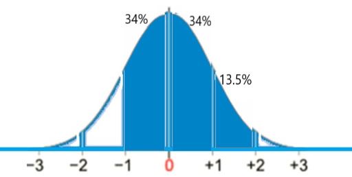
This gives P(40 < x < 70) = 34% + 34% + 13.5% = 81.5% (see below):

probability Of stocking out

If we stock out, demand is higher than supply. We stock 80 packs per week. This means that demand is higher than 80 packs that week:

• μ = 50, σ = 10, x = 80
• z = ^(80−50)/₁₀ = ³⁰/₁₀ = 3

This gives P(x > 80) = 0.15% (see below):

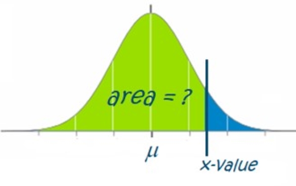
Calculating the Area Below an X-Value (Norm.DIST Exercise)

Let us now practice using Excel’s NORM.DIST() function to solve for probabilities. Remember the following is true when calculating the area below an [latex]x[/latex]-value:

For more precise area calculations or Areas that aren’t precisely 1, 2 or 3 standard deviations above or below the mean, Use Excel’s NORM.DIST() function P(X ≤ x) = NORM.DIST(x, μ, σ, 1) This gives the area to the left of x

Example 39.3.1

Problem Setup: A school’s SAT scores are normally distributed with a mean of 1,010 and standard deviation of 20.

Question: What percent of students have scores below 1,040 points?

You try 1: Drag the region we would highlight for this question onto the graph below:

You try 2: Select the correct Excel formula and resulting solution for this question:

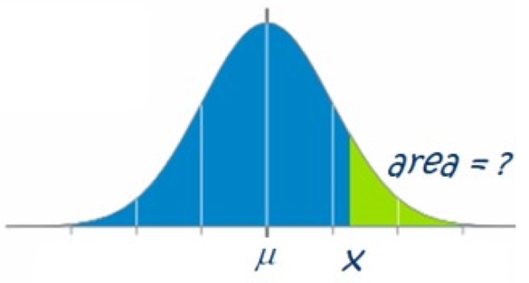
Calculating the Area Above an X-Value (Norm.DIST Exercise)

Remember, the following is true when calculating the area above an [latex]x[/latex]-value:

Excel’s NORM.DIST function returns the area to the left of x To calculate the area to the right, we take a complement P(X>x) = 1−NORM.DIST(x, μ, σ,1)

Example 39.3.2

Problem Setup: Let us keep going with our previous example of average SAT scores of 1,010 with a standard deviation of 20.

Question: What percent of students score above 1,040 on their SATs?

You try 1: Drag the region we would highlight for this question onto the graph below:

You try 2: Select the correct Excel formula and resulting solution for this question:

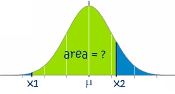
Calculating the Area Between Two X-Values (Norm.DIST Exercise)

Remember, the following is true when calculating the area between two [latex]x[/latex]-values:

To calculate the area between two x-values We need to deduct the area to the left of each x-value The remaining, middle area, will be the answer. P(x1≤x≤x2) = NORM.DIST(x2, μ, σ,1)−NORM.DIST(x1, μ, σ,1)

Example 39.3.3

Problem Setup: Let us, again, keep going with our previous example with average SAT scores of 1,010 with a standard deviation of 20.

Question: What percent of students score between 955 and 1,035 on their SATs?

You try 1: Drag the region we would highlight for this question onto the graph below:

You try 2: Select the correct Excel formula and resulting solution for this question:

Need more help? See the video in the section below for a full walk-through of these examples

Video & Additional Resources Explaining this section

Additional Resources:

• Click here to download the Powerpoint slides that accompany the video.
• Click here to download the Excel solutions for the Normal Distribution section.

Key Takeaways (EXERCISE)

Your Own Notes (EXERCISE)

• Are there any notes you want to take from this section? Is there anything you’d like to copy and paste below?
• These notes are for you only (they will not be stored anywhere)
• Make sure to download them at the end to use as a reference