Normal Distributions
Excel’s NORM.INV Function
Learning Objectives
Use Excel's NORM.INV() to calculate x-values related to given areas.
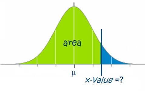
Left Area Given
 |
|
Right Area Given
 |
|
Middle Area Given
 |
|
Calculating the x-value for a left area (Exercise)
Let us first look at an example where we calculate an [latex]x[/latex]-value when the left area is given.
Example 40.1.1
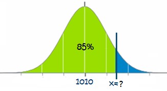
Problem Setup: Let us revisit the SAT score problem from the previous section. The average SAT score was 1,010 with a standard deviation of 20.
Question: What is the highest score for the bottom 85% of the students?
You try:
You try:
Conclusion: 85% of people score at most 1030.729 on their SATs.
Need Help? Go to the last section for a video that reviews all of the content in this section. You can also download a PowerPoint presentation on Normal Distributions.
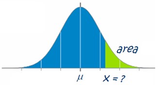
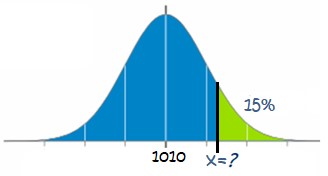
Calculating the x-value for a RIGHT area (Exercise)
Let us now look at an example where we calculate an [latex]x[/latex]-value when the right area is given.
Example 40.1.2
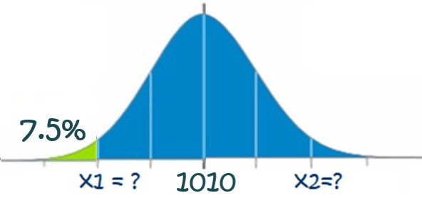
Problem Setup: Let us revisit the SAT score problem from the previous section. The average SAT score was 1,010 with a standard deviation of 20.
Question: Above what score do the top 15% of students score?
You try:
You try:
Conclusion: 15% of people score at least 1030.729 on their SATs.
Need Help? Click to reveal the solutions below OR go to the last section for a video explaining all content in this section.
Solutions To This Problem
When we are given the area to the right:
- We need to take a complement to get the area to the left
- This is because Excel's NORM.INV() function works with areas to the left
- So, for the top 15%, this is the same as the bottom 85%:
 |
 |
To calculate the [latex]x[/latex]-value associated with the above graphs, we use NORM.INV():
\[ x = \text{NORM.INV}(1-0.15,1010,20) = \text{NORM.INV}(0.85, 1010, 20) = 1030.729\]
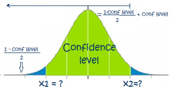
Calculating the x-values for a MIddle area (Exercise)
Let us finally look at an example where we calculate an [latex]x[/latex]-values when a middle area is given.
Example 40.1.3
Problem Setup: Let us revisit the SAT score problem from the previous section. The average SAT score was 1,010 with a standard deviation of 20.
Question: What is the range of SAT scores for the middle 85% of students?
You try:
You try:
You try:
You try:
You try:
Conclusion: 85% of students score between 981 and 1,038 on their SATs.
Need Help? Click to reveal the solutions below OR go to the last section for a video explaining all content in this section.
Solutions To This Problem
When we are given the middle area:
- We need to calculate the two [latex]x[/latex]-values separately
- Input the area to the left of [latex]x_1[/latex] and [latex]x_2[/latex] into NORM.INV
- The area to the left of [latex]x_1[/latex]: [latex]\frac{100\%-85\%}{2}=7.5\%[/latex]
- The area to the left of [latex]x_2[/latex]: [latex]\frac{100\%-85\%}{2}+85\%=92.5\%[/latex]
 |
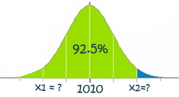 |
To calculate the [latex]x[/latex]-value associated with the above graphs, we use NORM.INV:
\[ x_1 = \text{NORM.INV}((1-0.85)/2,1010,20) = \text{NORM.INV}(0.075, 1010, 20) = 989.2713\]
\[ x_2 = \text{NORM.INV}((1-0.85)/2+0.85,1010,20) = \text{NORM.INV}(0.925, 1010, 20) = 1038.791\]
Video Explaining ALl topics in this section
Additional Resources:
- Click here to download the Powerpoint slides that accompany the video.
- Click here to download the Excel solutions for the Normal Distribution section.
Key Takeaways (EXERCISE)
Key Takeaways: Excel's NORM.INV Function
Drag the words into the correct boxes for each section below:
Click the sections below to reveal the solutions to the above exercises
Your Own Notes (EXERCISE)
- Are there any notes you want to take from this section? Is there anything you'd like to copy and paste below?
- These notes are for you only (they will not be stored anywhere)
- Make sure to download them at the end to use as a reference
