12.4 Integrated Rate Laws
Learning Objectives
By the end of this section, you will be able to:
- Explain the form and function of an integrated rate law
- Perform integrated rate law calculations for zero-, first-, and second-order reactions
- Define half-life and carry out related calculations
- Identify the order of a reaction from concentration/time data
The rate laws discussed thus far relate the rate and the concentrations of reactants. We can also determine a second form of each rate law that relates the concentrations of reactants and time. These are called integrated rate laws. We can use an integrated rate law to determine the amount of reactant or product present after a period of time or to estimate the time required for a reaction to proceed to a certain extent. For example, an integrated rate law is used to determine the length of time a radioactive material must be stored for its radioactivity to decay to a safe level.
Using calculus, the differential rate law for a chemical reaction can be integrated with respect to time to give an equation that relates the amount of reactant or product present in a reaction mixture to the elapsed time of the reaction. This process can either be very straightforward or very complex, depending on the complexity of the differential rate law. For purposes of discussion, we will focus on the resulting integrated rate laws for first-, second-, and zero-order reactions.
First-Order Reactions
Integration of the rate law for a simple first-order reaction (rate = k[A]) results in an equation describing how the reactant concentration varies with time:

where [A]t is the concentration of A at any time t, [A]0 is the initial concentration of A, and k is the first-order rate constant.
For mathematical convenience, this equation may be rearranged to a format showing a linear dependence of concentration in time:
The Integrated Rate Law for a First-Order Reaction:
The rate constant for the first-order decomposition of cyclobutane, C4H8 at 500 °C is 9.2 × 10⁻³ s−1:
How long will it take for 80.0% of a sample of C4H8 to decompose?
Solution:
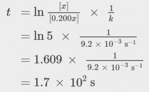
Since the relative change in reactant concentration is provided, a convenient format for the integrated rate law is:
The initial concentration of C4H8, [A]0, is not provided, but the provision that 80.0% of the sample has decomposed is enough information to solve this problem. Let x be the initial concentration, in which case the concentration after 80.0% decomposition is 20.0% of x or 0.200x. Rearranging the rate law to isolate t and substituting the provided quantities yields:
Check Your Learning:
Iodine-131 is a radioactive isotope that is used to diagnose and treat some forms of thyroid cancer. Iodine-131 decays to xenon-131 according to the equation:
The decay is first-order with a rate constant of 0.138 d−1. How many days will it take for 90% of the iodine−131 in a 0.500 M solution of this substance to decay to Xe-131?
16.7 days
In the next example exercise, a linear format for the integrated rate law will be convenient:
A plot of ln[A]t versus t for a first-order reaction is a straight line with a slope of −k and a y-intercept of ln[A]0. If a set of rate data are plotted in this fashion but do not result in a straight line, the reaction is not first order in A.
Graphical Determination of Reaction Order and Rate Constant:
The following data is for the decomposition of H2O2 at 40oC:
2H2O2 ⟶ 2H2O + O2
Show that the data can be represented by a first-order rate law by graphing ln[H2O2] versus time. Determine the rate constant for the decomposition of H2O2 from these data.
| Trial | Time (h) | [H2O2] (M) | ln[H2O2] |
|---|---|---|---|
| 1 | 0.00 | 1.000 | 0.000 |
| 2 | 6.00 | 0.500 | −0.693 |
| 3 | 12.00 | 0.250 | −1.386 |
| 4 | 18.00 | 0.125 | −2.079 |
| 5 | 24.00 | 0.0625 | −2.772 |
Solution:
The plot of ln[H2O2] is shown in (Figure).
![A graph is shown with the label “Time ( h )” on the x-axis and “l n [ H subscript 2 O subscript 2 ]” on the y-axis. The x-axis shows markings at 6, 12, 18, and 24 hours. The vertical axis shows markings at negative 3, negative 2, negative 1, and 0. A decreasing linear trend line is drawn through five points represented at the coordinates (0, 0), (6, negative 0.693), (12, negative 1.386), (18, negative 2.079), and (24, negative 2.772).](https://pressbooks.bccampus.ca/aperrott/wp-content/uploads/sites/1463/2021/07/CNX_Chem_12_04_FrstOKin-2.jpg)
The plot of ln[H2O2] versus time is linear, indicating that the reaction may be described by a first-order rate law.
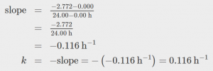
According to the linear format of the first-order integrated rate law, the rate constant is given by the negative of this plot’s slope.
The slope of this line may be derived from two values of ln[H2O2] at different values of t (one near each end of the line is preferable). For example, the value of ln[H2O2] when t is 0.00 h is 0.000; the value when t = 24.00 h is −2.772.
Check Your Learning:
Graph the following data to determine whether the reaction A ⟶ B + C is first order.
| Trial | Time (s) | [A] |
|---|---|---|
| 1 | 4.0 | 0.220 |
| 2 | 8.0 | 0.144 |
| 3 | 12.0 | 0.110 |
| 4 | 16.0 | 0.088 |
| 5 | 20.0 | 0.074 |
The plot of ln[A]t vs. t is not linear, indicating the reaction is not first order:
![A graph, labeled above as “l n [ A ] vs. Time” is shown. The x-axis is labeled, “Time ( s )” and the y-axis is labeled, “l n [ A ].” The x-axis shows markings at 5, 10, 15, 20, and 25 hours. The y-axis shows markings at negative 3, negative 2, negative 1, and 0. A slight curve is drawn connecting five points at coordinates of approximately (4, negative 1.5), (8, negative 2), (12, negative 2.2), (16, negative 2.4), and (20, negative 2.6).](https://pressbooks.bccampus.ca/aperrott/wp-content/uploads/sites/1463/2021/07/CNX_Chem_12_04_CYL1_img-2.jpg)
Second-Order Reactions
The equations that relate the concentrations of reactants and the rate constant of second-order reactions can be fairly complicated. To illustrate the point with minimal complexity, only the simplest second-order reactions will be described here, namely, those whose rates depend on the concentration of just one reactant. For these types of reactions, the differential rate law is written as:
For these second-order reactions, the integrated rate law is:

where the terms in the equation have their usual meanings as defined earlier.
The Integrated Rate Law for a Second-Order Reaction:
The reaction of butadiene gas (C4H6) to yield C8H12 gas is described by the equation:
This “dimerization” reaction is second order with a rate constant equal to 5.76 × 10⁻² L mol−1 min−1 under certain conditions. If the initial concentration of butadiene is 0.200 M, what is the concentration after 10.0 min?
Solution:
For a second-order reaction, the integrated rate law is written
We know three variables in this equation: [A]0 = 0.200 mol/L, k = 5.76 × 10⁻² L.mol-1.min, and t = 10.0 min. Therefore, we can solve for [A], the fourth variable:
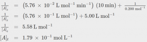
Therefore 0.179 mol/L of butadiene remain at the end of 10.0 min, compared to the 0.200 mol/L that was originally present.
Check Your Learning:
If the initial concentration of butadiene is 0.0200 M, what is the concentration remaining after 20.0 min?
0.0195 mol/L
The integrated rate law for second-order reactions has the form of the equation of a straight line:
A plot of 1/[A]t versus t for a second-order reaction is a straight line with a slope of k and a y-intercept of 1/[A]0. If the plot is not a straight line, then the reaction is not second order.
Graphical Determination of Reaction Order and Rate Constant:
The data below are for the same reaction described in (Figure). Prepare and compare two appropriate data plots to identify the reaction as being either first or second order. After identifying the reaction order, estimate a value for the rate constant.
Solution:
| Trial | Time (s) | [C4H6] (M) |
|---|---|---|
| 1 | 0 | 1.00 × 10⁻² |
| 2 | 1600 | 5.04 × 10⁻³ |
| 3 | 3200 | 3.37 × 10⁻³ |
| 4 | 4800 | 2.53 × 10⁻³ |
| 5 | 6200 | 2.08 × 10⁻³ |
In order to distinguish a first-order reaction from a second-order reaction, prepare a plot of ln[C4H6]t versus t and compare it to a plot of 1/[C4H6]t versus t. The values needed for these plots follow.
| Time (s) | 1/[C4H6] (M-1) | ln[C4H6] |
|---|---|---|
| 0 | 100 | −4.605 |
| 1600 | 198 | −5.289 |
| 3200 | 296 | −5.692 |
| 4800 | 395 | −5.978 |
| 6200 | 481 | −6.175 |
The plots are shown in (Figure), which clearly shows the plot of ln[C4H6]t versus t is not linear, therefore the reaction is not first order. The plot of 1/[C4H6]t versus t is linear, indicating that the reaction is second order.
![Two graphs are shown, each with the label “Time ( s )” on the x-axis. The graph on the left is labeled, “l n [ C subscript 4 H subscript 6 ],” on the y-axis. The graph on the right is labeled “1 divided by [ C subscript 4 H subscript 6 ],” on the y-axis. The x-axes for both graphs show markings at 3000 and 6000. The y-axis for the graph on the left shows markings at negative 6, negative 5, and negative 4. A decreasing slightly concave up curve is drawn through five points at coordinates that are (0, negative 4.605), (1600, negative 5.289), (3200, negative 5.692), (4800, negative 5.978), and (6200, negative 6.175). The y-axis for the graph on the right shows markings at 100, 300, and 500. An approximately linear increasing curve is drawn through five points at coordinates that are (0, 100), (1600, 198), (3200, 296), and (4800, 395), and (6200, 481).](https://pressbooks.bccampus.ca/aperrott/wp-content/uploads/sites/1463/2021/07/CNX_Chem_12_04_2OrdKin-2.jpg)
According to the second-order integrated rate law, the rate constant is equal to the slope of the 1/[A]t versus t plot. Using the data for t = 0 s and t = 6200 s, the rate constant is estimated as follows:
Check Your Learning:
Do the following data fit a second-order rate law?
| Trial | Time (s) | [A] (M) |
|---|---|---|
| 1 | 5 | 0.952 |
| 2 | 10 | 0.625 |
| 3 | 15 | 0.465 |
| 4 | 20 | 0.370 |
| 5 | 25 | 0.308 |
| 6 | 35 | 0.230 |
Yes. The plot of 1/[A]t vs. t is linear:
![A graph, with the title “1 divided by [ A ] vs. Time” is shown, with the label, “Time ( s ),” on the x-axis. The label “1 divided by [ A ]” appears left of the y-axis. The x-axis shows markings beginning at zero and continuing at intervals of 10 up to and including 40. The y-axis on the left shows markings beginning at 0 and increasing by intervals of 1 up to and including 5. A line with an increasing trend is drawn through six points at approximately (4, 1), (10, 1.5), (15, 2.2), (20, 2.8), (26, 3.4), and (36, 4.4).](https://pressbooks.bccampus.ca/aperrott/wp-content/uploads/sites/1463/2021/07/CNX_Chem_12_04_CYL2_img-2.jpg)
Zero-Order Reactions
For zero-order reactions, the differential rate law is:
A zero-order reaction thus exhibits a constant reaction rate, regardless of the concentration of its reactant(s). This may seem counterintuitive, since the reaction rate certainly can’t be finite when the reactant concentration is zero. For purposes of this introductory text, it will suffice to note that zero-order kinetics are observed for some reactions only under certain specific conditions. These same reactions exhibit different kinetic behaviors when the specific conditions aren’t met, and for this reason the more prudent term pseudo-zero-order is sometimes used.
The integrated rate law for a zero-order reaction is a linear function:
A plot of [A] versus t for a zero-order reaction is a straight line with a slope of −k and a y-intercept of [A]0. (Figure) shows a plot of [NH3] versus t for the thermal decomposition of ammonia at the surface of two different heated solids. The decomposition reaction exhibits first-order behavior at a quartz (SiO2) surface, as suggested by the exponentially decaying plot of concentration versus time. On a tungsten surface, however, the plot is linear, indicating zero-order kinetics.
Graphical Determination of Zero-Order Rate Constant:
Use the data plot in (Figure) to graphically estimate the zero-order rate constant for ammonia decomposition at a tungsten surface.
Solution:
The integrated rate law for zero-order kinetics describes a linear plot of reactant concentration, [A]t, versus time, t, with a slope equal to the negative of the rate constant, −k. Following the mathematical approach of previous examples, the slope of the linear data plot (for decomposition on W) is estimated from the graph. Using the ammonia concentrations at t = 0 and t = 1000 s:
Check Your Learning:
The zero-order plot in (Figure) shows an initial ammonia concentration of 0.0028 mol L−1 decreasing linearly with time for 1000 s. Assuming no change in this zero-order behavior, at what time (min) will the concentration reach 0.0001 mol L−1?
35 min
![A graph is shown with the label, “Time ( s ),” on the x-axis and, “[ N H subscript 3 ] M,” on the y-axis. The x-axis shows a single value of 1000 marked near the right end of the axis. The vertical axis shows markings at 1.0 times 10 superscript negative 3, 2.0 times 10 superscript negative 3, and 3.0 times 10 superscript negative 3. A decreasing linear trend line is drawn through six points at the approximate coordinates: (0, 2.8 times 10 superscript negative 3), (200, 2.6 times 10 superscript negative 3), (400, 2.3 times 10 superscript negative 3), (600, 2.0 times 10 superscript negative 3), (800, 1.8 times 10 superscript negative 3), and (1000, 1.6 times 10 superscript negative 3). This line is labeled “Decomposition on W.” A decreasing slightly concave up curve is similarly drawn through eight points at the approximate coordinates: (0, 2.8 times 10 superscript negative 3), (100, 2.5 times 10 superscript negative 3), (200, 2.1 times 10 superscript negative 3), (300, 1.9 times 10 superscript negative 3), (400, 1.6 times 10 superscript negative 3), (500, 1.4 times 10 superscript negative 3), and (750, 1.1 times 10 superscript negative 3), ending at about (1000, 0.7 times 10 superscript negative 3). This curve is labeled “Decomposition on S i O subscript 2.”](https://pressbooks.bccampus.ca/aperrott/wp-content/uploads/sites/1463/2021/07/CNX_Chem_12_04_AmDecomK-2.jpg)
The Half-Life of a Reaction
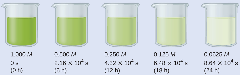
The half-life of a reaction (t1/2) is the time required for one-half of a given amount of reactant to be consumed. In each succeeding half-life, half of the remaining concentration of the reactant is consumed. Using the decomposition of hydrogen peroxide ((Figure)) as an example, we find that during the first half-life (from 0.00 hours to 6.00 hours), the concentration of H2O2 decreases from 1.000 M to 0.500 M. During the second half-life (from 6.00 hours to 12.00 hours), it decreases from 0.500 M to 0.250 M; during the third half-life, it decreases from 0.250 M to 0.125 M. The concentration of H2O2 decreases by half during each successive period of 6.00 hours. The decomposition of hydrogen peroxide is a first-order reaction, and, as can be shown, the half-life of a first-order reaction is independent of the concentration of the reactant. However, half-lives of reactions with other orders depend on the concentrations of the reactants.
First-Order Reactions
An equation relating the half-life of a first-order reaction to its rate constant may be derived from the integrated rate law as follows:

Invoking the definition of half-life, symbolized t1/2, requires that the concentration of A at this point is one-half its initial concentration: t= t1/2, [A]t = (1/2)[A]0.
Substituting these terms into the rearranged integrated rate law and simplifying yields the equation for half-life:

This equation describes an expected inverse relation between the half-life of the reaction and its rate constant, k. Faster reactions exhibit larger rate constants and correspondingly shorter half-lives. Slower reactions exhibit smaller rate constants and longer half-lives.
Calculation of a First-order Rate Constant using Half-Life:
Calculate the rate constant for the first-order decomposition of hydrogen peroxide in water at 40 °C, using the data given in (Figure).
Solution:
Inspecting the concentration/time data in (Figure) shows the half-life for the decomposition of H2O2 is 2.16 × 10⁴ s:

Check Your Learning:
The first-order radioactive decay of iodine-131 exhibits a rate constant of 0.138 d−1. What is the half-life for this decay?
5.02 d.
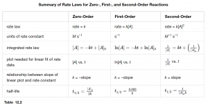
Equations for the half-lives of zero- and second-order reactions can be derived, but will not be covered in this course. Equations for both differential and integrated rate laws and the corresponding half-life for first-order reactions are summarized in (Figure).
 Key Concepts and Summary
Integrated rate laws are mathematically derived from differential rate laws, and they describe the time dependence of reactant and product concentrations.
The half-life of a reaction is the time required to decrease the amount of a given reactant by one-half. A reaction’s half-life varies with rate constant and, for some reaction orders, reactant concentration. The half-life of a first-order reaction is independent of concentration.
Key Equations
- integrated rate law for zero-order reactions: [A]t = −kt + [A]0,
- integrated rate law for first-order reactions: ln[A]t = −kt + ln[A]0,
- half-life for a first-order reaction: t1/2 = 0.693/k,
- integrated rate law for second-order reactions: ,
Glossary
- half-life of a reaction (tl/2)
- time required for half of a given amount of reactant to be consumed
- integrated rate law
- equation that relates the concentration of a reactant to elapsed time of reaction
