56 EWE book testing – Villy Christensen

Source: https://pressbooks.bccampus.ca/ewemodel/chapter/introduction-to-ecospace/

About Ecospace

The Ecospace model is a spatially explicit time dynamic model based on the Ecopath mass-balance and Ecosim time dynamic routines ^{[1] [2]}. It applies the same set of differential equations as used in Ecosim, executed for each cell in a grid of cells. In Ecosim, a set of differential equations is defined based on the biomass change during time for consumer functional groups, expressed as

()  

where B_it is the biomass of i at time t, g_i is the growth efficiency, I_i is the immigration rate; F_it is the mortality rate due to harvesting (fishing mortality); e_i is the emigration rate; and M0_i the other mortality (mortality not explained in the model). The terms Q_ij and Q_ji represent the consumption due to predation by i on j, and by j on i, respectively. For primary producers, the term f (B_it)) represents the growth term as function of the group biomass ^[3].

The consumption rates Qij are based on the foraging arena theory (see chapter), where the biomass of prey i is split between a vulnerable (V_ij) and a non-vulnerable (B_i-V_ij) component. The transfer rate, called vulnerability (υ_ij) between the two fractions determines the vulnerable biomass at time interval dt:

where a_ij is the effective search rate for the predator j, and h_j is handling time for the predator. The vulnerability parameter υ_ij is a function of the maximum increase in predation mortality under the given predator/prey conditions (see vulnerability multiplier chapter). High values of υ_ij imply large proportions of biomass (B_i) vulnerable to predator j (V_ij), and thus imply V_ij = B_i, and that the predator j is far from its carrying capacity with regards to prey i.

In Ecospace, the spatial extent of the ecosystem is represented by a grid of cells, each of which can be defined as land or water and, and have a habitat type assigned to the cell. Ecospace represents the biomass (B) and consumption (Q) dynamics over a two-dimensional space as well as time ^[4]. Space, time, and state are considered discrete variables by using the Eulerian approach, which treats movements as ‘flows’ of organisms among fixed spatial reference cells.

In the original Ecospace model ^[5], a first step of parameterizing entails the definition of a basemap based on habitat information (depth strata, bottom type, etc.) in the study area. Species preferences are then assigned to these habitat types based on the biology and ecology of the species included in each functional group of the ecosystem model, their depth distributions, their preferred sediment type, etc. In addition, the original Ecospace model required for habitat definitions,

1. the dispersion rate of each functional group in ‘preferred’ habitats,
2. the relative dispersal rate in ‘non-preferred’ habitats, and
3. the relative feeding rate in non-preferred habitat by functional group.

Fishing fleets can be depicted as operating in a specific region and cells can be defined as protected areas.

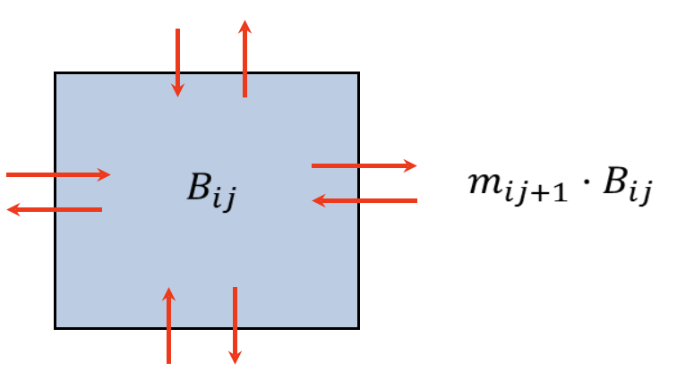
Figure 1. For each cell, the inbound dispersal rate I_i is the sum of emigration flows from the four surrounding cells, while the outbound instantaneous dispersal rates m_i from a given cell in Ecospace vary based on the pool type, cell conditions/habitat, and response of organisms to predation risk and feeding conditions

Moreover, relative variations of primary productivity and fishing costs can be defined for the initial conditions of the model. For trophic interactions, fishing, and movement calculations, biomass is considered as homogeneous within each cell and movement of biomass and flows is allowed across the borders to adjacent cells. For each cell, the immigration rate I_i of Eq. ?? is assumed to consist of up to four emigration flows from the surrounding cells (Figure 1). The emigration flows (B_out,rci) are in turn similarly represented as instantaneous movement rates m_i times the biomass density in the cell (B_rci):

where (rci) represents cell row and column for group i, and d is movement direction (up, down, left or right).

The instantaneous emigration rates m_i from a given cell in Ecospace are assumed to vary based on the functional group, habitat preferences, and responses of organisms to depredation risk and feeding conditions. The probability of movement of organisms towards favourable habitats was in the original Ecospace formulation calculated by means of a ‘habitat gradient function’ for each mapped habitat type and species or group i. Biomass dynamics in unsuitable cells were modified by predicting higher rates of emigration, lower feeding rates, and/or higher vulnerability to predation, a complex gradient calculation to modify dispersal rates is used to direct biomass toward suitable cells.

In more recent versions of Ecospace, a habitat capacity model has been included to estimate cell-specific continuous habitat suitability factor, where the area that species can feed in each cell is determined by functional responses to multiple environmental factors. See the habitat capacity chapter.  It is optional whether to use a habitat and/or habitat suitability for any given group, though in many recent applications habitat suitability is used predominantly while habitats mainly are used for defining where fleets can operate.