45 Introduction to Ecospace

Setting the stage

Marine ecosystems are complex systems affected by the state of the environment and a myriad of human activities. The full impact of these human activities on the complex ecosystem are becoming more critical to understand, and are now requested by agencies concerned with numerous policies and strategies that involve spatial management actions (in Europe, for instance by the Common Fisheries Policy, Marine Strategy Framework Directive, Farm to Fork, Zero Pollution and Biodiversity Strategies). All of these have divergent end-points, but all require an understanding of how multiple forms of human activities impact marine ecosystems. To better manage our impact on marine ecosystems, and notably consider trade-offs in management, there is a need to advance scientific capabilities to provide both quantitative descriptions and quantitative evaluations of the effect of spatial management interventions, factoring in plausible future changes in climate and human activities.

Spatial-temporal ecosystem modeling has grown in capacity, complexity, and focus to undertake such complex tasks, and is increasingly considered an indispensable tool to contribute to policy and management, including multi-sectoral Ecosystem Based Management (EBM) and Marine Spatial Planning (MSP).

Among the tools available, the temporal and spatial dynamic model EwE approach is of special interest for its wide range of applications across ecosystem types. Ecospace has notably been used to contribute to EBM, most often to a subset of EBM, Ecosystem-Based Fisheries Management, or EBFM. Applications of Ecospace include the evaluation of spatial trophic interaction patterns, modeling of species distribution based on habitat suitability, the assessment of Marine Protected Area (MPA) placement and connectivity, harvest allocations and, more recently, environmental impact analysis and the assessment of episodic mortality events, effects of changes in nutrient inputs, climate change, and cumulative impacts (e.g.,^{[1] [2] [3] [4] [5] [6] [7] [8] [9] [10] [11] [12] [13] [14] [15] [16] [17] [18]}.

The development of Ecospace has involved an evolutionary process where many additional capabilities have been developed over the years in response to requests by users. The more recent advancements include the Habitat Foraging Capacity Model (HFC^[19])and the Spatial Temporal Data Framework (STDF^[20]), which have enabled Ecospace applications to fully consider climate variability and change, taking into account different types of uncertainty^[21] [22]. These innovations and a substantial increase in the various applications of EwE^[23], provided a call for an update of the Ecospace, which led to a book chapter by de Mutsert et al.^[24] upon which a number of the chapters in the present text book are based (as attributed). The present text book and the EwE User Guide seek to present the most up-to-date guidelines for using and understanding Ecospace’s capabilities and challenges.

About Ecospace

The Ecospace model is a spatially explicit time dynamic model based on the Ecopath mass-balance and Ecosim time dynamic routines^{[25] [26]}. It applies the same set of differential equations as used in Ecosim, executed for each functional group and cell in a grid of cells. In Ecosim, a set of differential equations is defined based on the biomass components of change for consumer functional groups, expressed as

[latex]\frac{dB_i}{dt}=g_i\cdot\sum\limits_{j=1}^{n}Q_{ji}-\sum\limits_{j=1}^{n}Q_{ij}+I_i-(F_{it}+e_i+M0_{it})\cdot B_{it}\tag{1}[/latex]

where B_it is the biomass of i at time t, g_i is the growth efficiency, I_i is the immigration rate; F_it is the mortality rate due to harvesting (fishing mortality); e_i is the emigration rate; and M0_i the other mortality (mortality not explained in the model). The terms Q_ji and Q_ij represent the consumption due to predation by j on i, and by i on j, respectively. For primary producers, the consumption rate term is replaced by a production rate function f (B_it)) represents primary production rate as a function of the group biomass^[27]; that function is nonlinear, representing competition effects for light and nutrients.

The consumption rates Q_ji are predicted using equations from foraging arena theory (see chapter), where the biomass of prey i is split between a vulnerable (V_ij) and a non-vulnerable (B_i-V_ij) component.  The vulnerability exchange parameters used in predicting the various Q_ji mainly represent spatial distribution and movement behaviors at very fine scales, typically far smaller than the size of Ecospace spatial grid cells.

In Ecospace, the spatial extent of the ecosystem is represented by a grid of cells, each of which can be defined as land or water, and each cell can have characteristics or attributes like a habitat type. Ecospace then represents the biomass (B) and consumption (Q) dynamics over a two-dimensional space as well as time^[28]. Space, time, and state are considered discrete variables by using the Eulerian approach, which treats movements as "flow" of organisms among fixed spatial reference cells.

In the original Ecospace model^[29], a first step of parameterizing entailed the definition of a base map based on habitat information (depth strata, bottom type, etc.) in the study area. Species preferences were then (and still can be if more elaborate spatio-temporal habitat use functions are not used) assigned to these habitat types based on the biology and ecology of the species included in each functional group of the ecosystem model, their depth distributions, their preferred sediment type, etc. In addition, the original Ecospace model required for habitat definitions,

1. the dispersal (spatial mixing) rate of each functional group in "preferred" habitats,
2. the relative dispersal rate in "non-preferred" habitats, and
3. the relative feeding rate in non-preferred habitat by functional group.

Fishing mortality rate for each cell can represent effects of fishing effort by multiple fishing fleets, and each fishing fleet can be depicted as operating in a specific region and habitat type, and cells can be defined as protected areas for particular or all fishing fleets.  Fishing effort is assumed to move between grid cells over time in response to spatial and temporal variation in profitability of fishing.

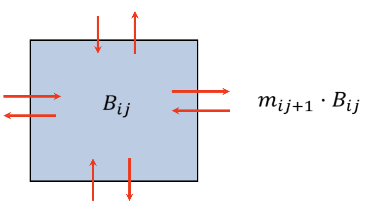
Figure 1. For each cell, the inbound dispersal rate I_i is the sum of emigration flows from the four surrounding cells, while the outbound instantaneous dispersal rates m_i from a given cell in Ecospace make up the basic Ecosim emigration rates e_i, and vary based on the pool type, cell conditions/habitat, and response of organisms to predation risk and feeding conditions.

Moreover, spatial variations of primary productivity and fishing costs can be defined as initial conditions for the basic model.

For trophic interactions, fishing, and movement calculations, biomass is considered as homogeneous within each cell and movement of biomass and flows is allowed across the borders to adjacent cells. For each cell, the immigration rate I_i of Eq. 1 is assumed to consist of up to four emigration flows from the surrounding cells (Figure 1). The emigration flows (B_out,rci) are in turn similarly represented by instantaneous movement rates m_i times the biomass density in the cell (B_rci) with the sum of those loss rates like m_i,j+1 representing the emigration rate e_i in eq. 1:

[latex]B_{out,rci}=\sum\limits_{d=1}^{4}m_{id}\cdot B_{rci} \tag{3}[/latex]

where (rci) represents cell row and column for group i, and d is movement direction (up, down, left or right).

The instantaneous emigration rates m_i,d from a given cell in Ecospace are assumed to vary based on the functional group, habitat preferences, and can be set to vary with trophic conditions within each cell (to model responses of organisms to predation risk and feeding conditions). The probability of movement of organisms towards favourable habitats was in the original Ecospace formulation calculated by means of a "habitat gradient function" for each mapped habitat type and species or group i. Biomass dynamics in unsuitable cells were modified by predicting higher rates of emigration, lower feeding rates, and/or higher vulnerability to predation, and a complex gradient calculation continues to be used so as to modify dispersal rates to cause higher movement rates of biomass toward suitable cells.

In more recent versions of Ecospace, a habitat capacity model has been included to estimate cell-specific continuous habitat suitability factors where the area that species can feed in each cell is determined by functional responses to multiple environmental factors^[30]. See the habitat capacity chapter.  It is optional whether to use a habitat and/or habitat suitability for any given group, though in many recent applications habitat suitability is used predominantly while habitats mainly are used for defining where fleets can operate.

The very large equation system represented by eq. 1 with mixing terms is solved numerically on one month time steps using an implicit integration method (BDF2, second order backward differentiation), that works very well for long-lived species but tends to predict short lived species to change more slowly than Ecosim predicts.  As in Ecosim, the Ecospace BDF integration does not "see" the very rapid boom-bust dynamics that can be exhibited by groups with high P/B (e.g. phytoplankton and short-lived zooplankters), but instead predicts an average biomass for these groups.

For advanced applications involving multi-stanza groups, there are two Ecospace option^[31].  The first "multi-stanza" solution option. is to keep track of overall multi-stanza numbers at age over the map while predicting local variation in abundance from concentration patterns predicted from spatial m_ij variations of the differential equation system.  The second or "IBM" option is to divide the multi-stanza recruitment numbers at each time step into a large number of packets of individuals, then simulate random and directed movements of these packets over the map as the organisms grow.  Details of the IBM equations are presented later in the chapter on Spatial implementation of multi-stanza and IBM.