27 Bout feeding

Many predators do not feed continuously over time as assumed in derivation of the vulnerable abundance Va in the standard foraging arena equation (Eq. 1 below).  Rather, they obtain most of their food intake in short, intensive feeding “bouts”, typically at dawn and dusk when light levels are changing rapidly^{[1] [2]}.

Particularly when predators such as juvenile fish have severely restricted habitat use as a tactic for managing predation risk (hiding, schooling), only a small fraction of the system-scale prey biomass is available to them in the foraging arenas that they use during each feeding bout. As an example, juvenile Atlantic salmon have been shown to restrict the time they spend feeding rather than maximizing their growth when food is abundant^[3].

Here, we show that overall trophic flow rates Q_ak (for predators k feeding in foraging arena a) over longer time scales can still be closely approximated by a continuous rate equation of the mass-action form Q_ak = α_akV_i(a)P_k(a), where the bout search rates α* and mean vulnerable prey densities per feeding bout are comparable to (but differ numerically from) the α,V predictions for continuous feeding.

Consider a single feeding bout in arena a of duration d (d << one day), during which an initial prey density V_a(0) is depleted by predators k(a).  Assume that d is short enough that prey renewal and loss during the bout, (e.g., due to prey spatial movement and other mortality sources) can be safely ignored.  Assume that V_a(0) is a proportion f_a of total prey biomass B_i(a) and that renewal mechanisms between bouts make V_a(0) = f_a B_i(a).  Note that when used over multiple bouts, this prediction of V_a(0) for each bout requires that arena prey abundance be independent of predation effects in previous bouts except through effects on B_i(a), i.e. that there are no carryover effects from previous bouts (extreme opposite of continuous feeding assumption).  Then if predators k search randomly within the arena, vulnerable prey density V_a(t) will change during the bout according to the simple rate equation,

[latex]\frac{dV_a(t)}{dt}=-V_a(t)\sum \limits_k\alpha_{ak}P_k\tag{3}[/latex]

where the α_ak are predator rates of effective search with the same interpretation as for continuous feeding.

Integrating Eq. 3 over the bout duration d leads to the familiar exponential exploitation equation V_a(d) = V_a(0) exp(-d ∑_k α_ak P_k) and to predicted total prey consumption per bout Q_ak^bout by each predator k,

[latex]Q_{ak}^{bout}=\frac{\alpha_{ak}P_k}{\sum\limits_k\alpha_{ak}P_k}\cdot f_aB_{i(a)}\cdot [1-\exp(-d\sum\limits_k\alpha_{ak}P_k)]\tag{4}[/latex]

The first term of Eq. 4 simply apportions total prey consumption V_a(0) – V_a(d) over the bout among competing predators.  Further, the mean prey density V_a^* during the bout is given by the integral of V over the bout divided by bout duration d. This mean is just,

[latex]V_a^*=f_aB_{i(a)}\cdot \frac{1-\exp(-d\sum\limits_k\alpha_{ak}P_k)}{d\sum\limits_k\alpha_{ak}P_k}\tag{5}[/latex]

Expressed in terms of this mean arena prey density, consumption per bout Eq. 4 can be expressed more simply as

[latex]Q_{ak}^{bout}=\alpha_{ak}P_kV_a^*\tag{6}[/latex]

We could use this formula directly in a complex simulation model that steps forward in time by the interval Δ_t between feeding bouts, adding in other components of prey and predator abundance change over each such short interval.  Fortunately, such a tedious calculation is generally unnecessary.

Consider the component of overall prey biomass change caused by each feeding bout, where there are n_b = 1/Δ_t bouts per year.  That (typically small) change in B_i(a) per bout is given by the sum of Eq. 4 terms over predators k, i.e.,

[latex]\Delta B_{i(a)} = f_aB_{i(a)}\cdot[1-\exp(-d\sum\limits_k\alpha_{ak}P_k)]\tag{7}[/latex]

Dividing this by the bout duration Δ_t gives a discrete-time component of the prey rate of change,

[latex]\frac {\Delta B_{i(a)}}{\Delta t}=\frac{1}{\Delta t}f_aB_{i(a)}\cdot [1-\exp(-d\sum\limits_k\alpha_{ak}P_k)] =n_bf_aB_{i(a)}\cdot [1-\exp(-d\sum\limits_k\alpha_{ak}P_k)]\tag{8}[/latex]

Since the time Δ_t between bouts is typically very short (n_b is typically of the order of several hundred bouts per year), we can approximate Eq. 8 very accurately by treating it as a continuous rate component dB_i(a)/dt.  This approximation leads immediately to a continuous rate equation for Q_ak comparable to the continuous feeding case where Q_ak = α_akP_kV_a, namely,

[latex]Q_{ak}=\alpha_{ak}^* \ P_k \ v_a^* \ B_{i(a)}\cdot \frac{1-\exp(-\sum\limits_k\alpha_{ak}^*P_k)}{\sum\limits_k\alpha_{ak}^*P_k}=\alpha_{ak}^* \ P_k \ V_a^*\tag{9}[/latex]

Where α_ak* are the duration-weighted search rates α_ak* = α_akd. v_a* = n_b f_a represents a total prey “fraction” that would become vulnerable over a one-year time scale, and  V_a* (comparable to Eq 2) is given by

[latex]V_a^*=v_a^* \ B_{i(a)} \cdot \frac{1-\exp(-\sum\limits_k\alpha_{ak}^* \ P_k)}{\sum\limits_k\alpha_{ak}^* \ P_k}\tag{10}[/latex]

This model for vulnerable prey density obviously exhibits the same “ratio dependence” of available prey density on predator abundance as does Eq 2, but with the ratio effect 1/(v+v’+∑_k α_ak P_k) replaced by a negative exponential effect.   At high predator abundances it also implies an upper bound B_i(a) on total removal rate Q_a and hence on total instantaneous predation mortality rate Q_a/B_i(a).

We can parameterize the continuous approximation to bout feeding from Ecopath inputs and assumed maximum predation rates in the same way as described in the previous section for continuous arena feeding.  That is, we set v_a* = K_a M_a(0) where K_a as above is a defined input ratio of maximum to Ecopath baseline predation rate.  We calculate base mean prey density per bout V_a*(0) by substituting Ecopath base prey and predator abundances B_i(a)(0) and P_k(0) into Eq. 10 along with ∑_k α P_k(0) = Q_a(0) / V_a(0), (where Q_a(0) is the base total consumption rate summed over predators k), and solving for V_a*, to give

[latex]V_{a}^*(0)=-\frac{Q_a(0)}{\ln(1-\frac{1}{K_a})}\tag{11}[/latex]

Then we simply calculate the α_ak* as

[latex]\alpha_{ak}^*=-\frac{Q_{ak}(0)}{P_k(0)\cdot V_a^*(0)}\tag{12}[/latex]

whereas above the arena-specific base consumption rate is calculated using assumed arena feeding proportions p_ak as Q_ak(0) = p_akQ_i(a),k(0), and Q_i(a),k(0) is the Ecopath base total consumption rate of prey i(a) by predator k.

Figure 1. Comparison of instantaneous mortality rates expressed relative to Ecopath baseline predation mortality rates for the original model formulation (“Continuous”) and compared to bout feeding with v_a* = v_a in case Bout A, and with v_a* < v_a set to give same limiting maximum consumption per predator, Q/P in case Bout B.

It is instructive to compare the predictions of instantaneous prey mortality rate M = Q_a/B_i(a) from Eq. 8 to those of the continuous model defined by Eq. 2  (and Q_a = ∑_k α_ak P_k V_a), for varying predator abundances P_k while holding prey biomasses B_i(a) constant (Figure 1). If we set v_a* = v_a, i.e. use the same K_a to calculate v_a* as we would for v_a in the continuous case (Bout A in Figure 1), the exponential term in the bout feeding model generally predicts steeper variation in M than the continuous model, i.e., it predicts that M will drop off more rapidly if P decreases from P(0) than does the continuous model.  This leads to weaker “compensation” measured in terms of increase in potential Q/P as P declines.  But if we set v_a* smaller than v_a, so as to predict the same limiting maximum consumption per predator (Q/P) at very low predator densities (Bout B in Figure 1), the two arena models give predicted patterns of variation in M that are the opposite, i.e. bout feeding predicts saturation of M at lower P than the continuous case.  This means that in Ecosim cases where K_a has been estimated by fitting the continuous arena model to time series data (the only option before the inclusion of bout feeding in EwE), and where feeding in reality has been of the bout type, the fitted K_a estimates have probably been somewhat too large, i.e K_a is in reality closer to 1.0 and predators are already causing (in the Ecopath base situation) what may be close to their maximum possible predation rates from bout feeding.

For Ecosim models that include multi-stanza population dynamics, a critically important capability is to represent adjustments in foraging time, particularly for juvenile stanzas.  Such adjustments allow juvenile fish to translate increases in potential feeding rate Q/P into reduced foraging time and predation risk when competitor abundance P decreases^[4], leading to compensatory changes in juvenile mortality rates and emergent stock-recruitment relationships of the Beverton-Holt form^[5].

Foraging time adjustments are modeled in Ecosim by including a dynamic variable T_i for each biomass type, with T_i at time zero set to 1.0.  Then T_i is varied over time so as to try and maintain Ecopath base feeding rate per predator (Q/P), by multiplying all search rates of type i for its prey by T_i, and all vulnerability exchange rates of type i into arenas where predators take it by T_i.  In the bout foraging representation, this means simply that (1) search parameters for type i as a predator are adjusted by varying bout durations d in proportion to T_i (i.e. setting α*(t) = α*(0) T_i, with T_i defined as the relative bout duration d(t)/d(0)) and (2) the vulnerable fraction f that define v* of i to its predators are also treated as being proportional to d by setting v*(t) = v*(0) T_i.

As a simple test of whether bout feeding is likely to make much difference to the ability of Ecosim models to fit historical time series data, we examined changes in a simple fitting criterion (sum of squared deviations, SS, from historical data, summed over all time series used in model fitting) for a collection of models that had been fitted to data using the continuous arena equations, when all trophic linkages were simply reset to assume bout feeding without correction or refitting of the K_a parameters (Figure 2,^[6]). Ability of several of these models to fit historical data are reviewed in Walters and Martell (2004, Figure 12.6^[7]), and these were mostly the same models used in single-species versus multispecies MSY comparisons by Walters et al.^[8].

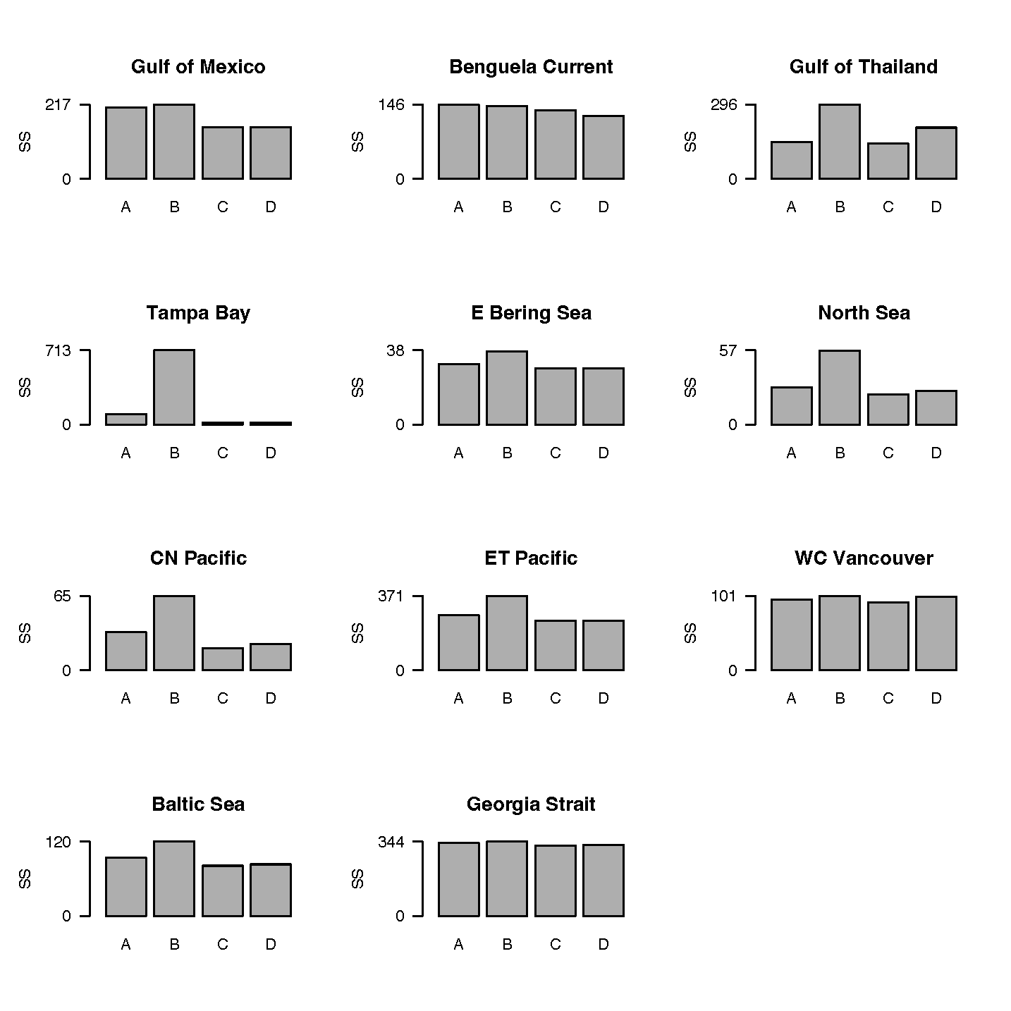
Surprisingly, there was little change in the fitting criterion for many of the models, and one (Central North Pacific) even gave a better fit immediately.  For those models where there was a substantial increase in SS, it was easy to remedy the poor fits by re-estimating K_a under the global bout arena assumption.  When we refitted the models under both feeding assumptions (by nonlinear estimation search over the 20 K_a values with largest contributions to the sum of squares), we were easily able to find fits at least as good under the bout feeding assumption for most cases, and qualitatively as good for all cases.

Discussion

The equations introduced here obviously give considerable flexibility to represent trophic interactions in the Ecosim model more realistically than previously possible^[9].  It is particularly comforting to see that the much more realistic assumption of bout rather than continuous feeding leads to very similar predictions of how prey mortality rates should vary with predator abundances as have been assumed in previous Ecosim models based on the unrealistic but mathematically convenient assumption of continuous feeding with rapid equilibration of vulnerable prey densities.

We recommend extreme care in using either the continuous or bout feeding equations to represent feeding by multiple predators in a relatively small number of arenas.  As noted above, the intense inter-specific competition implied by such concentration of feeding has very likely driven natural selection for differentiation in feeding behavior (use of different fine-scale arenas) as well as in diet composition.  See for instance Berec et al. (2006) for an experiment illustrating this. If such differentiation is excluded from the model parameterization, the Ecosim user risks building a model that will not retain observed biodiversity over time.

A few authors have referred to the basic Ecosim equation for predicting total flow rates Q =(α v B P) / (v + v’ + α P) as though it were a functional response equation comparable to assuming mass-action encounters and type II predation, e.g., Q =(α B P) / (1 + h B);^[10].  Such comparisons reflect a misunderstanding about a basic proposition of foraging arena theory, namely that predators very generally encounter their prey in space-time restricted circumstances (foraging arenas), such that it is almost never appropriate to predict Q from the ecosystem-scale mean prey density B when trying to account for effects such as handling time and switching (changes in α).  We would argue that it is sometimes appropriate to account for handling time effects, but only if these are predicted using arena-scale vulnerable prey densities V, i.e. Q = α V P / (1 + hV), where V is adjusted away from the system-scale average B using assumptions about localization of foraging (effects of vulnerability exchanges v’s and/or available prey fractions per bout f’s in the arena equations). We explicitly allow switching in Ecosim, but again caution that it should be used in conjunction with predictions of vulnerable, rather than overall, prey densities.

It would be ignorant to assert that the equations presented in this chapter are the only or best way to represent differentiation of vulnerable prey biomasses V from system-scale average prey biomasses B in prediction of trophic interaction rates.  They do not for example account explicitly for some very gross system-scale effects that occur in highly disturbed systems, such as changes in overall prey and predator distributions and overlap patterns, (e.g., due to range contractions), and changes in spatial arena structure due to obvious habitat changes like growth and destruction of biogenic spatial refuges^[11].  Some such changes can be accounted for in Ecosim through trophic ‘mediation functions’ that link v’s and α’s to abundances of species besides those engaged directly as predators and prey, (e.g., one can make α’s and v’s for juvenile fish that hide in macrophyte beds dependent on macrophyte biomass).  But there is still a long way to go in development of fully-defensible predictions of V for systems that are massively disturbed.

One option for dealing with the prediction of V would be to construct very detailed spatial models (with habitat and its use modelled at fine scale, maybe of a few m²) running on very short (bout) time scales (time steps of one hour or less).  But such models may be plagued by lack of detailed spatial data, lack of understanding of how organisms move and concentrate their activities at such fine scales, and risk of cumulative divergence of predictions from reality simply due to explosions over simulated time and space of small errors in behavioural movement predictions.

A key advantage of the relatively simple foraging arena equations for Q prediction is that we can easily force them to agree with baseline “observations” or estimates of system-scale abundances (B’s, P’s), feeding rates, and diet compositions (Q_ji) as summarized in static (point-in-time) mass-balance assessments like Ecopath.  But this is also a disadvantage, in the sense that the rate parameter estimates then become dependent on the often incomplete and possibly biased estimates entered as Ecopath inputs.  It is clear that Ecosim-type dynamic predictions are sensitive to those baseline inputs, and that this represents an especially severe issue for interactions involving small fish as prey (where the small fish typically represent only trivial and often overlooked proportions of their predators’ diets).

Even absent difficulties with Ecopath inputs, i.e. empirical knowledge of baseline ecosystem biomass flow rates and states, the most troublesome parameters for Ecosim users to specify have been the “vulnerability multipliers” K_a representing ratios of maximum to Ecopath base predation mortality rates.  One source of trouble is obviously that Ecopath inputs provide no information about the K_a, and such information can only come from either fine-scale analysis of spatial arena structures, from data collected at different times and/or places about how Q’s have varied with predator and prey abundances, or from assumptions about or estimates of where populations are relative to their carrying capacity.  Indeed, this is why we emphasize the importance of fitting Ecosim models to time series data by varying the Ka parameters.

Another, and important aspect is that the K_a are not purely “behavioural” or ecological parameters; rather, they depend as well on how large the Ecopath initial predator abundances P_k are compared to what the ecosystem might naturally support (see Density dependence chapter).  So for example a model that includes Atlantic cod stocks off Newfoundland, and uses the current low stock size as the Ecopath base, must have very high K_a values (1000+) for interactions between cod and its prey, else the model will not make enough prey available to the simulated cod stock for it to recover to anywhere near its historical abundance when simulated fishing is removed.

We can provide some guidance about reasonable ecological Ka values (corrected for effects of historical depletion on biomasses) from meta-analysis of K_a estimates for many fitted models.  One pattern that is becoming broadly evident from cases like those in Figure 2 is that fitted K_a values tend to be small (<2.0) for most trophic linkages in temperate and tropical systems, and for feeding by juvenile stanzas in all systems.  In contrast, fitted K_a values tend to be much larger for most interactions (except juvenile stanzas of demersal fish species) in high-latitude ecosystems like the Bering Sea.  The low K_a values are easily explained for juvenile fish and reef-associated older fish, as a consequence of severe spatial restriction in habitat use leading to low proportions of prey populations being available the fish at any time^[12].  High K_a values in high-latitude systems likely reflect the wider spatial movement characteristic of northern fish, and tactics such as diel vertical migration that bring high proportions of widely distributed predators and prey into daily contact with one another, (i.e., high f’s for bout feeding during periods of diurnal contact^[13]).

The K_a vulnerability multipliers are discussed in details in the vulnerability multiplier chapter.