Tutorial: Price elasticity

We will, once again return to Anchovy Bay where anchovy are caught by seiners and bait boats, In spite of the name of the second fleet, the anchovy from both fleets are primarily used for human consumption. The bait boats land high-quality anchovy, and have a secondary market supplying anchovy for recreational fisheries and a lobster trap fishery (not in the model).  Because of the high quality, the bait boats average €3/kg for anchovy, which is more than the €2/kg that seiners command. Anchovy is popular as a tasty, healthy and economic fish to buy in the fresh fish supply. But there is a limit to how much can be sold as there are no exports, so it’s only the local markets that have demand. The implication of this is that the price for anchovy is impacted by supply, which we can introduce in the model through price elasticity.

We can use any version of the Anchovy Bay model that you may have or you can download it from this x.

Open the model, go to Ecosim and do a run (Ecosim > Output > Run Ecosim > Run), check the model output to acquaint yourself with the model.

Next, let’s change the model slightly so that we can get more anchovy from it. Go to Ecosim < Input < Fishing effort, click on Trawlers at the lower panel, and then Set to value, enter 5 to increase trawler effort five times throughout the Ecosim run. Do the same for Seiners, also five times increase. This change is to fish out whiting and mackerel, the major predators on anchovy to allow for a build-up of anchovy that can sustain a higher fishing pressure. Run Ecosim (Ecosim > Output > Run Ecosim > Run), see Figure 1.

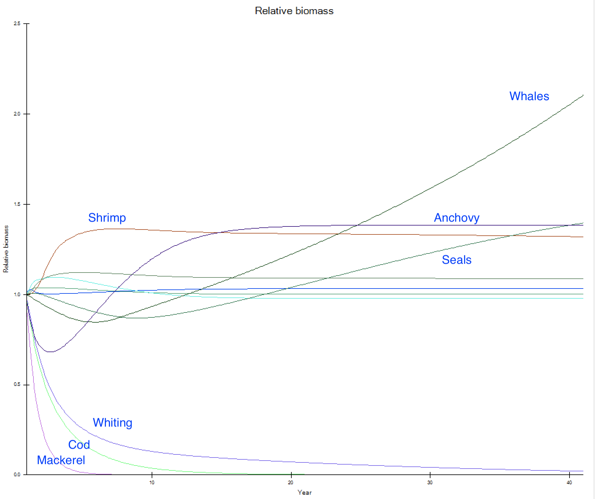
Figure 1. Ecosim run with five times increase in effort for Seiners and Bait boats. Notice how the anchovy biomass initially declines, then increases beyond the baseline in spite of higher fishing pressure. This shows predator release. 

Next, go to Ecosim > Output > Ecosim results > Group landed by: and extract the anchovy catches and values for Seiners and Bait boats.  Store these values for later.

Open the Ecosim > Input > Price elasticity form, and Add a shape. If you’ve worked with Mediation, you may notice that the setup is very similar (though the shapes are green – the colour of money, some say), and programmatically the price elasticity form is indeed derived straight from the Mediation form.  Click Change shape set Shape type to Linear and set Start to 1 and End to 0.1. Hopefully, you’ll now have a shape like in Figure 2.

Figure 2. Price elasticity shape defined on the Ecosim > Input > Price elasticity form. 

In the Figure 2 shape, note that there is a vertical stippled blue line. That line sets where on the figure the Ecopath baseline situation is. That is, when the landings are at that level the landing price(s) will be the same as entered in the Ecopath baseline (€2/kg and €3/kg, for anchovy landed by seiners and bait boats, respectively).  The default placement of the vertical blue line is at ⅓ of the X-axis, and in this example the value there is 0.7 x the max value. If landings increase 3 times, the Y-axis value will be reduced to the minimum value of 0.1, and it will remain for any higher catch level. Does that seem reasonable = what you want? If not, you can use your mouse to move the vertical blue line to the left or right as you see fit. Just remember that the vertical line represents your baseline and ask what will happen if catches change.

The linear shape in Figure 2 is an approximation that is not data-driven, but a quick and easy way to explore the impact of price elasticity. You could dive and perhaps find data – do that for a real application.^[1]

We now have a shape, but need to define what it represents. Click Define supply on the Price elasticity form and the Define supply form pops up (Figure 3).

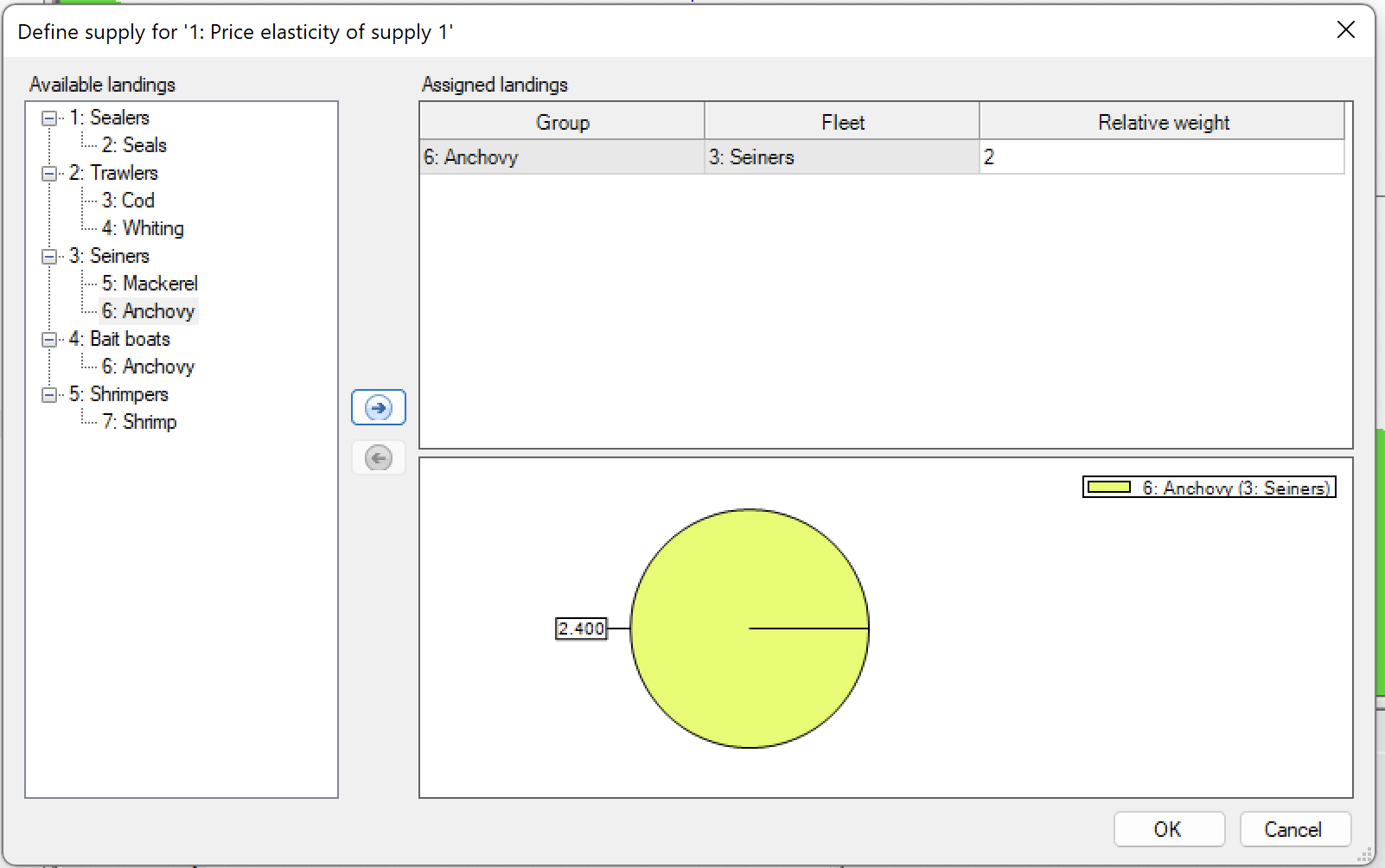
Figure 3. Define supply form for price elasticity. Under Seiners click Anchovy and then the arrow-right button to transfer Seiners > Anchovy to the Assigned landings. Press OK.

Assign the Seiners > Anchovy landings to drive the price elasticity from as shown in Figure 3. Note that the relative weight is the unit landing price for the group. This is of relevance where you have more than one group driving the price elasticity. In that case  the default assumption is that the overall measure of landing capacity if a function of the value of each of the groups being landed.  That’s an assumption, replace it with data, where possible (if not, it’s a reasonable default assumption).

Next we need to apply the function, this is done at the Ecosim > Input > Price elasticity > Apply price elasticity form, see Figure 4. Follow the instructions in the figure legend.

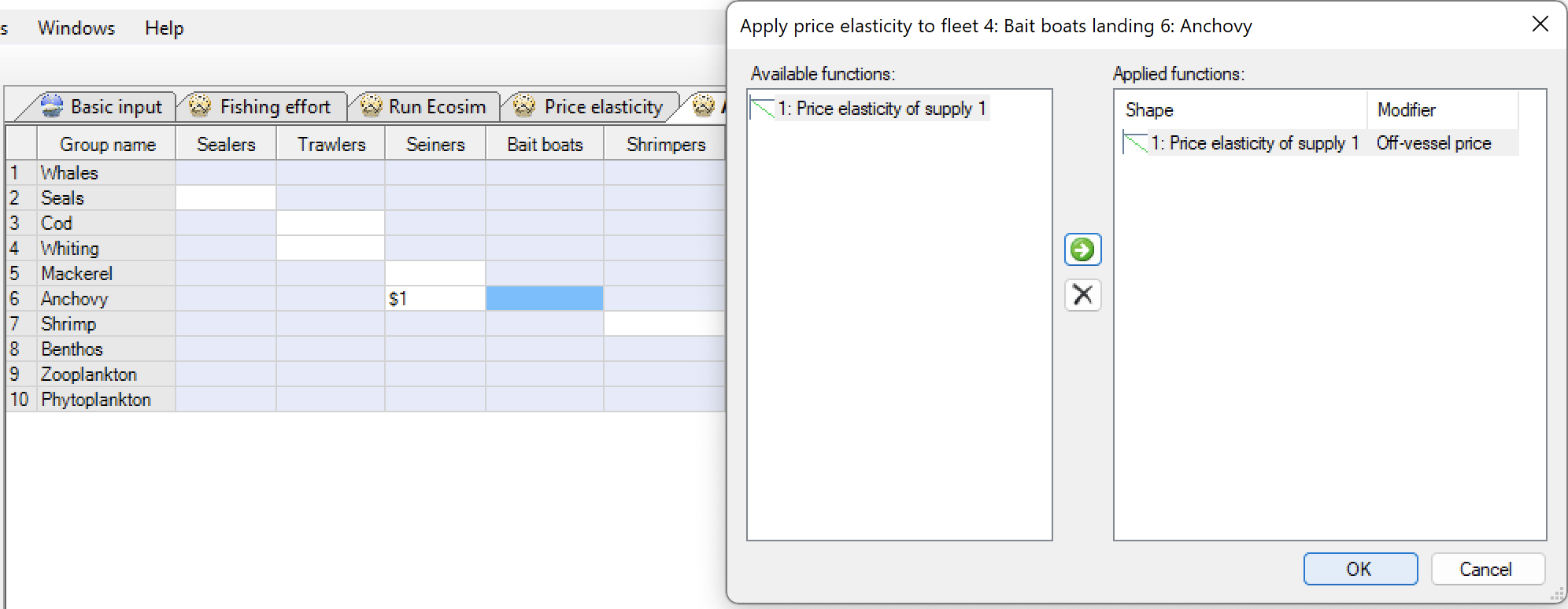
Figure 4. Apply price elasticity form. One by one, click the intersection between Seiners or Bait boats vs. Anchovy, and on the pop-up form use the right-arrow to apply the functions, and press OK. The figure shows the second of intersections (Baits boats and Anchovy) being applied. Once completed, there should be $1 (for first price elasticity function) for anchovy for boat fleets. 

Notice that it is the landings of anchovy from the seiners fleet that drives the price elasticity function, but that the impact of this is being used for anchovy from both the seiners and the bait boats. Is that logical? Perhaps not, but the bulk of the catch come from the seiners, and bait boat delivers a high quality specialty product. But the main purpose of this is really just to demonstrate that it possible to have landing prices for one fleet being a function of another fleet’s landings – think for instance about the potential case of surimi production impacting pricing for king crab.

You should now have the complete setup of price elasticity for the Anchovy Bay model. When you run economic routines, e.g., the value chain or policy optimization, the landing price of anchovy will be a function of the landings. But here, we’ll simply extract the value of the landings from a standard Ecosim run.

Run the Ecosim model again (Ecosim > Output > Run Ecosim > Run), and you’ll hopefully find that the run looks exactly like it did the first time we ran Ecosim in this tutorial (similar to Figure 1). That’s because price elasticity only changes the value of the landings in this case, so the runs are identical. If you instead were doing policy optimizations with value as an objective, the runs, i.e. the optimum would be different.

Again, extract the anchovy catches and values from the Ecosim results form (Ecosim > Output > Ecosim results > Group landed by:).

• Compare the anchovy landings, are they the same with and without price elasticity?
• What about the anchovy values?

There more about price elasticity in the preceding chapter and in the EwE User Guide.