26 Shared foraging arenas

The basic Ecosim formulation for predation interactions assumes that each non-zero consumption of a prey type i by a predator type j takes place in a foraging arena unique to that interaction^{[1] [2] [3]}.  The rationale for this assumption is that each arena is defined by the combined behaviors of both the prey and the predator, and possibly also by selection of particular prey sub-types, (e.g., sizes), such that multiple predators can feed on the same prey type in different ways (at different depths, times of day, spatial microhabitats) without competing directly for prey within the typically very confined space represented by each arena.

The general foraging arena assumption that predation typically is concentrated within restricted arenas, and hence at restricted rates, has profound implications for model predictions about ecosystem stability, and the further assumption that each predator-prey interaction takes place within a unique arena has equally profound implication for the maintenance of ecosystem structure and diversity^[4].  It essentially represents the possibility of a distinct “feeding niche” for each of the predators that takes type i prey, hence allowing for the possibility that multiple predators can coexist while feeding on only that prey type.  A prototype example of this possibility is with rockfishes (Sebastes spp.) along the Pacific coast, where a diverse collection of species all feed on euphausids, but avoid direct competition for these euphausids by feeding at different depths and times of day.  An obvious evolutionary argument in favour of assuming such fine structure in feeding interactions is that if several predators were to feed within the same micro-scale foraging arena, the intense inter-specific competition caused by such behavior would result in very strong natural selection favouring differentiation of behaviors to avoid it, e.g., by feeding at different depths or times.

While there are evolutionary arguments in favour of assuming a distinct foraging arena for every interaction, Aydin and Gaichas^[5] emphasize that there are some situations where multiple predator types are likely to feed on exactly the same prey and at the same place and time.  An example could be where the predator types represent different life history stanzas (age-size classes) of the same predator species with very similar feeding modes (times and locations).

We represent this possibility in Ecosim by entry of base proportions of each predator type’s diet that occurs in each of the possible foraging arenas defined by all non-zero predator-prey consumption linkages.  Vulnerable prey density in each arena is then represented as varying over time in response to abundances of all predator types that feed in the arena.

In Ecosim, we define a list a = 1, … , N_a of possible foraging arenas, where N_a is the number of non-zero consumption interactions in the Ecopath diet matrix representing consumption of each prey type i by predator type j.  Each of these potential arenas has a defining prey type i(a) and defining predator type j(a).

When only predator type j(a) feeds in arena a, vulnerable prey density V_a is predicted by the basic foraging arena equation,

[latex]V_a=\frac{v_a \cdot B_{i(a)}}{v_a+v_a' +\alpha_a \cdot P_{j(a)}}\tag{1}[/latex]

Here, v_a and v_a‘ are vulnerability exchange rates of prey to and from arena a, B_i(a) is prey biomass, P_j(a) is predator abundance (biomass or sum of numbers times search rates per  predator for multi-stanza predators), and α_a is the predator rate of effective search (volume swept per time divided by foraging arena volume).  The predation flow rate (biomass of prey i(a) consumed per unit of time by predator j(a)) is then predicted as Q_i(a),j(a) = α_aV_aP_j(a).  The v_a and α_a are parameterized by having model builders define va from maximum possible mortality rates expressed as multiples K_a of Ecopath base instantaneous predation rates M_ij⁽⁰⁾ = Q_ij⁽⁰⁾ / B_i⁽⁰⁾, simply by setting v_a = K_a where the superscript (0) designates Q’s and B’s estimated as base (initial) values of abundances and flows in the Ecopath baseline model.  The back-exchange parameter v’ is set equal to v since it cannot be estimated separately from the α_a parameter.

The shared-arena extension of Eq. 1 is straightforward,

[latex]V_a=\frac{v_a \cdot B_{i(a)}}{v_a+v_a'+ \sum \limits_k \alpha_{ak} \cdot P_k}\tag{2}[/latex]

Here the predator impact on V_a is represented by a sum over all possible predators k of arena-specific search rates α_ak times predator abundances P_k. [In the software-implementation of this, we do not actually sum over all k but instead construct a list of all non-zero α_ak flow combinations, and sum the α_akP_k denominator terms only over the elements of that list.]

To parameterize Eq. 2 in a relatively simple way while assuring that it predicts predation rates equal to Ecopath base rates when the system is at its Ecopath base state, we need to specify base proportions p_ak of each predator k’s diet that is taken in arena a. These proportions are constrained to sum to Ecopath base consumption rates  over all a for which i(a) = i.  That is, we take the by-arena base flows  to be p_ak Q_i(a),k⁽⁰⁾.  These base flows then imply a base instantaneous mortality rate M_a⁽⁰⁾ totaled over predators feeding in a, for prey i(a),

[latex]M_a^{(0)}=\frac{\sum \limits_k Q_{ak}^{(0)}}{B_{i(a)}}\tag{3}[/latex]

Using this input or baseline estimate of M for each arena and an assumed vulnerability multiplier K_a for that arena, we simply set v_a = K_a (and v_a‘ = v_a).

Next, note that to be consistent with Ecopath baseline inputs, we must require that Ecosim predict Q_ak⁽⁰⁾ when all biomasses (and p’s) are at their Ecopath base values. The Ecosim prediction of rate Q_ak (flow rate of prey to predator k from feeding in arena a) at any time is Q_ak = α_akV_aP_k, implying we must constrain the α_ak so that Q_ak⁽⁰⁾ = α_ak V_a⁽⁰⁾ P_k⁽⁰⁾, i.e. we must set α_ak = Q_ak⁽⁰⁾ / (V_a⁽⁰⁾ P_k⁽⁰⁾ ).  This means that to estimate the α_ak we must first estimate the base vulnerable abundances V_a⁽⁰⁾.

This estimation turns out to be remarkably simple, when we note that the Ecopath base value of ∑_k α_ak P_k must equal ∑_k Q_ak⁽⁰⁾ / V_a⁽⁰⁾, (simply sum Q_ak over k, which must equal Va = ∑_k α_ak P_k, and solve for ∑_k α_ak P_k). Substituting ∑_k Q_ak⁽⁰⁾ / V_a⁽⁰⁾ for ∑_k α_ak P_k in Eq. 2, then solving for V_a⁽⁰⁾, we calculate the base vulnerable abundances to be simply,

[latex]V_a^{(0)}= v_a \cdot B_{i(a)} - \frac{\sum \limits_k Q_{ak}^{(0)}}{v_a+v_a'}\tag{4}[/latex]

The α_ak are then calculated from these base vulnerable biomasses. Time-varying values of Q_ak are computed efficiently in Ecosim by setting up a list h = 1, … , N_h of all non-zero by-arena flows (N_h ≥ N_a), where for each list element we store its associated prey type i(h), predator type k(h), and arena a(h).

To calculate Q_ak, we sweep down this list repetitively.  On the first sweep, we accumulate the denominator sums ∑_k α_ak P_k for Eq. 2.  We then sweep down the arena list and calculate V_a for every a again using Eq. 2.  Then we sweep again down the h list, calculating Q_ak = α_akV_aP_k and accumulating predictions of total predation rates on the prey i(a) and food consumption rates by predators k(a).

As an added bit of model realism, one can specify a non-zero prey handling times for predator k (type II functional response^[6]), and the Q_ak calculation is modified to be Q_ak = (α_ak/H_k) V_a P_k, where H_k is the denominator of Holling’s multi-species disc equation for predator k feeding.  This handling time correction is also applied in the bout-feeding formulation described in the next chapter.

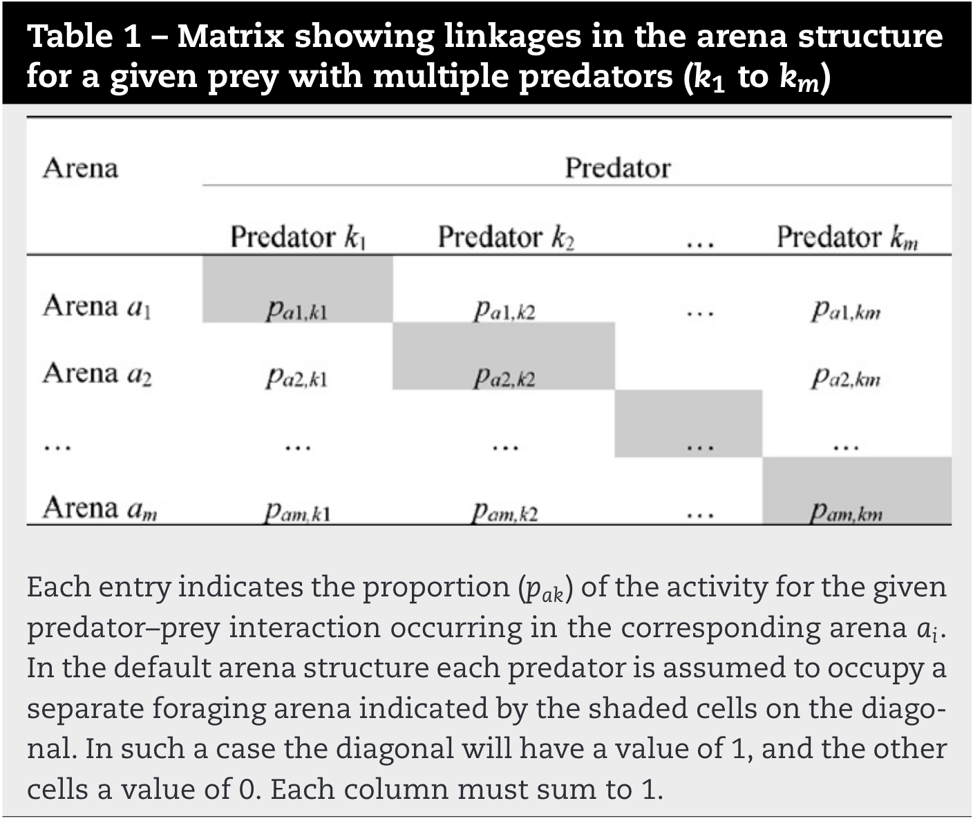
To edit the p_ak diet proportions array, we display a matrix for each prey type i of the non-zero i-k consumption proportions, as shown schematically in Table 1. In this table, m is the number of non-zero flows from prey ito predators k where each such flow defines a potential foraging arena.  Note that each column of the table must sum to 1.0, i.e. all of the consumption by predator kj of prey type i must be accounted for by feeding in one of the m identifiable arenas for prey type i.  The Ecosim default proportions for this table imply that each predator takes all of its consumption of prey type i in a unique arena, i.e. the table is an identity matrix, (with values of 1 on the shaded diagonal in Table 1).

The opposite extreme of this default assumption would be that all consumption of prey type i by its predators occur in only one arena or behavioral state for prey i, as shown in Table 2. This case implies maximum possible impact of predators k on availability of prey i to one another, and will cause competitive exclusion of at least some predator types in Ecosim unless the predators are well-differentiated in terms of overall diet composition, i.e. where each predator “specializes” on a different prey type i, which dominates the diet composition, as for instance shown by Schmidt^[7]. Studies rather tend to indicate resource partitioning between competing predator species, leading to non-additive mortality rates, see e.g., Griffen and Byers^[8]. Separation where diet compositions indicate predator overlap may also be caused by temporal exclusion of prey based on availability to the predator^[9].

In the special case where a set of predators feeds on only one prey type in a single arena (Table 2), and where there are no complications such as multistanza population dynamics where abundance of one or more predator types may be limited by recruitment rates from younger stanzas, the above formulation implies that there is not even a unique equilibrium point for predator abundances.  Rather, all predator abundance combinations that predict V=V(0) in Eq. 2 are neutral stable points provided predator mortality rates remain at Ecopath base values, such that any temporary pulse of differential mortality that causes one or more predators to decline will then be followed by persistence of the new predator abundance combination if mortality rates return to the base values.  Any predator that suffers a persistent differential increase in mortality rate is predicted to decline toward extinction.