50 Migration and advection

Ecospace dynamically allocates biomass across a grid map while accounting for mixing rates between adjacent grid cells.  In the simplest cases, the basic assumptions about these rates are,

1. they are symmetrical from a cell to its four adjacent cells if all four cells have equal habitat capacity,
2. which is modified whether a cell is defined as “preferred habitat” or not (running means over adjacent sets of five cells allows for smooth transitions between habitat types), and
3. user-defined increased predation risk and reduced feeding rate in non-preferred habitat.

Additionally, Ecospace can simulate advection of biomass for organisms that drift passively with surface currents, and also seasonal migrations of organisms that move over large distances within each year.  For multi-stanza groups, an additional option (see Ecospace IBM chapter) allows division of each monthly cohort into a large number of packets, with movement of these packets simulated as a stochastic process so as to potentially generate realistic patterns of movement (and possibly migration) of organisms of different ages.

Representing seasonal migration in Ecospace

Larger organisms commonly have seasonal migration patterns that allow them to utilize favourable seasonal resource and environmental conditions over large spatial areas. Such movements can be represented in Ecospace in two ways. First is using a simple “Eulerian” approach, which involves explicitly modelling changes in instantaneous rates of biomass mixing among the Ecospace spatial cells, in some way that approximates at least the changing center of distribution of the migratory species.  The second way is the “Lagrangian” approach, which is for multi-stanza groups only. It simulates stochastic movements of a large number of “individuals”, i.e packets of biomass that move together over the spatial map.

The Eulerian approach is implemented in Ecospace by allowing users to define a monthly sequence of “preferred” position map cells (or clusters of cells) by first declaring which groups that are migratory on the Ecospace > Input > Dispersal form, then on the Ecospace > Input > Maps form sketch (or import) for each month the preferred cells for each migration group.

The Migration dialogue box displays a map of the Ecospace region, with migratory species, month by month over a calendar year. Preferred position for each month (and the annual trajectory of preferred positions) is set by setting a value on the interface and sketching the area of distribution

Figure 1. Migration input at Ecospace > Input > Maps.

Double-clicking on the selected functional group name (“Whales” in Figure 1), will bring up a spreadsheet with the migration values. These can be imported and exported, and thus derived externally for more reproducible behaviour.

The mathematical method used in Ecospace to create migratory behaviour is quite simple. Spatial movement is represented in general in Ecospace as a set of instantaneous exchange rates across the boundaries of adjacent spatial cells. For migratory species, these exchange rates are simply multiplied by relative factors at each simulation time step, where the factors depend on distance from the preferred cell for that time step as shown in Figure 2. The function is reversed for movement across a northern cell boundary. A similar function is used for east-west movements with map column-preferred column as the independent variable.

The factor has no effect (multiplies movement rates by 1.0, so movement rates are similar in all directions) for cells near the preferred cell (or cluster of cells), and “shuts down” movement away from the preferred cell for cells far from that preferred cell. Note that the base movement rates that are multiplied by the migration factors may not be the same in all directions to start with; these base rates can include advection effects and/or increased/oriented movement rates towards preferred habitats. That is, migration effects can be combined with advection and orientation of movement toward preferred habitats; it was the intention to represent such combined effects that motivated the multiplicative factor formulation in the first place.

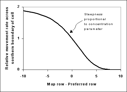
Figure 2. Relative movement rates; see text for details.

Tips for setting up migration in Ecospace

Unfortunately, there is no way to make the Ecospace migration simulations very simple to set up, particularly when using the IBM option to simulate movement more realistically for multi-stanza groups. Generally one must do considerable numerical experimentation to find reasonable migration parameter values and a stable numerical solution scheme. These cannot be computed in advance since they depend on a variety of details about the spatial map grid and species movement characteristics. Here are a few key points to keep in mind while experimenting (by repeated simulations) with the migration interface:

• The concentration parameters are relative values that the user needs to set by trying alternatives (generally in the range 0.5 to 4.0) to see what values give general distribution patterns similar to those observed in the field. Low values (<1.0) lead to weak distortion of movement toward preferred cells and hence to more widely spread distributions, while high values (e.g. 3.0) give distributions strongly concentrated near the preferred cells.
• Mean annual movement distances (Ecospace > Input > Dispersal form) have to be set large enough for migrating species to be able to “track” movements in preferred locations. As a general rule, set the base dispersal rate for migratory species to at least 100L km/year, where L is mean body length in cm.  This is particularly critical for multi-stanza groups where different stanzas commonly reside in non-overlapping areas, and may need to move considerable distances during each “ontogenetic habitat shift” (without suffering too high relative predation risk or poor feeding rate conditions).
• Setting high concentration parameter values (>2.0) and/or moving animals through a very complex map with many coastal blocking features can result in numerical instability in the Ecospace solution algorithm. The best way to correct this is to reduce the movement distances somewhat; it may also be necessary to reduce the Successive over-relaxation (SOR) weight (Ecospace > Input > Ecospace parameters form) used in solving the linear equations involved in the numerical scheme for integrating the spatial rate equations (implicit method, BDF2 backward differentiation that is most often stable but can be problematic when there are very strong spatial gradients).
• Setting high concentration parameter values can also result in “overfishing”. Ecospace allocates total fishing effort over the map proportional to the total number of cells initially used by each fishing fleet,  so when the model generates a concentrated distribution of some favoured species, the total effort will concentrate accordingly and can sometimes generate very high fishing rates near the center of the migrating stock distribution. Remedies include reducing total effort by reducing the total efficiency multiplier (Ecospace > Input > Ecospace fishery > Fleet dynamics > Tot. eff. multiple. ) and distributing effort more widely (reduce value of “effective power” on the same form).

• Concentrating a migratory predator can cause local depletion of food organisms and/or reduced per- predator feeding rates due to prey vulnerability limits. If these effects cause simulated total predator biomass to incorrectly decline over time (and if the user determines that the declines are not due to an artifactual overfishing effect), then it may be necessary to either increase total prey abundances (in Ecopath) or vulnerability of prey to the predator (Ecosim > Input > Vulnerability multipliers form).
• Multi-stanza population dynamics may behave strangely or incorrectly when one or more life history stages are migratory while other(s) are not. Ecospace does not keep track of the full population age/size distribution for each spatial cell (prohibitive memory and computing time requirement), and instead updates only the total abundances by stanza then distributes those using either the non-stanza prediction of biomass distribution or the IBM packet simulation approach. Either approximation tends to “dampen” abundance fluctuations in the early life history stanzas that might be created by, for example, seasonal movement of the adults to spawning locations near preferred juvenile habitats.

Advection in Ecospace

Advection processes are critical for productivity in most ocean areas. Currents deliver planktonic production to reef areas at much higher rates than would be predicted from simple turbulent mixing processes. Upwelling associated with movement of water away from coastlines delivers nutrients to surface waters, but the movement of nutrient rich water away from upwelling locations means that production and biomass may be highest well away from the actual upwelling locations. Convergence (down-welling) zones represent places where planktonic production from surrounding areas is concentrated, creating special opportunities for production of higher trophic levels.

Once an advection pattern has been defined, the user can specify which biomass pools are subject to the advection velocities (vu,vv field) in addition to movement caused by swimming and/or turbulent mixing. This allows examination of whether some apparent “migration” and concentration patterns of actively swimming organisms, (e.g., tuna aggregations at convergence zones) might in fact be due mainly to random swimming combined with advective drift.

Older versions of Ecospace had an interface that allowed users to “sketch” simple advection patterns which were then corrected to insure mass balance (or allowed to exhibit areas of upwelling and downwelling into depths not modeled by Ecospace).  That method never worked well, and we advise users to work with advection fields calculated with credible and well-tested hydrodynamic models.

Output from hydrodynamic models can be used as time-varying spatial input for Ecospace via the Temporal Spatial Framework of EwE, see the EwE User Guide for details.