Tutorial: Caesium in Anchovy Bay
William Walters
This tutorial can be developed in an Excel spreadsheet to solve for the parameters needed for input into Ecotracer. The tutorial is based on a rather typical situation where there are not reported values for all parameters, and it is necessary to make estimates for missing parameters.
The base Ecopath model is Anchovy Bay, in a version that you can download from this link (along with the spreadsheet than can be used as guidance for the tutorial, see details below. We advice though that you create your own spreadsheet and set up the needed calculations, as described).
Concentration ratios are usually reported in the literature, or have to be derived from separately reported studies for water concentrations and for concentrations in biota. Typically, assuming no temperature, particles (salts), or pressure effects, 1 m3 of water is here assumed equal to 1 t (in reality, it is slightly more than 1 t because of notably dissolved salt). Measurements of the contaminant in biota need to be scaled to the biomass unit in Ecopath (t km-2, which when multiplied by area in km2 yields t) as they are usually reported per gram of tissue. Measurements of a contaminant in dry weight should be changed to wet weights using a conversion factor.
Table 1. List of symbols used.
- Elimination rates (Ke; day‐1)
| Symbol | Description | Unit |
| Bi | Biomass | tonne |
| P/Bi | Production to biomass ratio | year‐1 |
| TLi | Trophic level | unitless |
| CRi | Concentration ratio | unitless |
| CREwEi | EwE concentration ratio | unitless |
| Ke
mi |
Elimination rates
Excretion rate |
day-1
year‐1 |
| di | Decay rate | year‐1 |
| AEi | Assimilation efficiency | 0 ‐ 1 |
| ui | Direct absorption rate | km2∙t∙year‐1 |
| Ai,eq | Equilibrium amount | g |
| Ci,eq | Equilibrium concentration | g∙t‐1 |
Table 2. Starting data for an Ecotracer simulation of 137Cs with data concerning Ecopath parameters (B, TL, and P/B) from the Anchovy Bay model and data representative of what might be measured in field surveys or reported in the literature. The table is designed to replicate an Excel spreadsheet. Values needed to be transferred into the Ecotracer routine include the excretion rate (mi), physical decay rate (di), the amount not assimilated (1‐AE), amount of 137Cs (Ai). Methods need to be used to estimate missing values of mi, Ai, 1AE, and transforming the environmental concentration from a volume to spatial basis. Ui is solved by finding total gains (TGains) from consumption (Cons) and direct uptake (DU), and total losses (TLoss) from Losses and Ai.

Note: A spreadsheet with Table 2 (Ecotr-sprdsheet tab) is included in the zip file with the database.
Starting Information
Ecotracer and all values can be done in a spreadsheet to find missing values. The intent of this scenario is to build a spreadsheet model for all the parameters to run in Ecotracer. The parameters for the Ecopath model (B, P/B, and TL) are taken from the Anchovy Bay model with additional ecotoxicological data being provided. For our purposes, we will arbitrarily consider Anchovy Bay to be 1000 m x 1000 m with an average depth of 250 m. 137Cs in Anchovy Bay has been found to have an activity of 2 Bq∙m‐3.
The following represents a way to estimate the direct absorption rate for groups. Generally, for substances that bioaccumulate, the amount of a substance such as 137Cs in a group or species is more dependent on diet than direct uptake at higher trophic levels.However, the direct absorption rate is an important parameter to estimate throughout the food web. Lack of a direct absorption rate at lower trophic levels can lead to an overestimate on the importance of diet or to an error being amplified through the food web with higher trophic levels not reaching measured or likely concentration levels.
- The average of 2 Bq∙m‐3 needs to be converted to Bq∙km‐2. The volume of the ocean is calculated as 250,000,000 m3 leading to 500,000,000 Bq∙km‐2.
- Elimination rates (Ke; day‐1) need to be determined for groups that lack data. In this scenario log Ke is plotted against the TL of groups to estimate the Ke for groups that lack data (Figure 1). The resulting relationship is used to estimate the Ke for the groups that lacked data. The Ke is then used to estimate (Ke x 365) the excretion (= elimination) rate (mi; year‐1).
- Loss rates in this example result from total mortality (P/B), physical decay rates (di), and elimination rates (mi) and these can be summed to be applied against the amount (Ai) of 137Cs in the groups.
- Assimilation efficiencies for groups missing data need to be estimated. In this simulation, since all fish groups had an AE of 0.8, and given AEs range between 0.75 and 0.95 a value of 0.8 was used for fish and invertebrate groups without a reported AE. For marine mammals the AE is calculated from the total gains and total losses (i.e., AE = Total losses/Total gains).
- Concentrations (Bq∙t‐1) are needed to estimate the direct absorption rate for all groups excluding marine mammals. In this scenario there are three groups without concentration data. Therefore, in this simulation a regression analysis is done plotting concentration against trophic level (Figure 2). The importance of estimating a direct absorption rate is for simulations done when there are changing environmental concentrations or changes to the underlying Ecopath input parameters.
- Calculating the gains from consumption in order to solve for ui. Recall that at equilibrium when dCi(t)/dt = 0, that the gains are equal to the losses. We have set up the loss rate (step 3), and the gains, excluding marine mammals, are both due to the direct absorption rate (from step 5) and consumption gains. Consumption gains are estimated from AEi, Qi (consumption), and Aj/Bj (concentration in diet items of predator i). Unfortunately, the concentration of detritus is not known, but it is derived from all the unassimilated consumption from the Ecopath model. As a result, it is an iterative process that involves an estimate of what the concentration in detritus would be. Generally, a good guess is to start with phytoplankton as it is a large contributor to detritus; in Anchovy Bay, phytoplankton contribute approximately 70 % of the flow to detritus. Thus, starting detritus with the same concentration as phytoplankton to determine the ui for all groups, and then run Ecotracer to get the estimate of the concentration of 137Cs for detritus. Then re‐run with the new concentration for detritus.
- Before the second iteration it is necessary to re‐calculate the gains from consumption; if the Excel spreadsheet is set up with formulas this will change the values of ui as well. This example started with a value of 16 Bq∙t‐1 for detritus, and after the first run Ecotracer estimated 22.4 Bq∙t‐1. Using this value for the second iteration and after changing the consumption values and ui for the groups the second iteration estimated a value of 21.92 Bq∙t‐1 (close enough!).

Figure 1. Relation between the elimination rate constant (Ke) and trophic level used to estimate the elimination rate (mi).
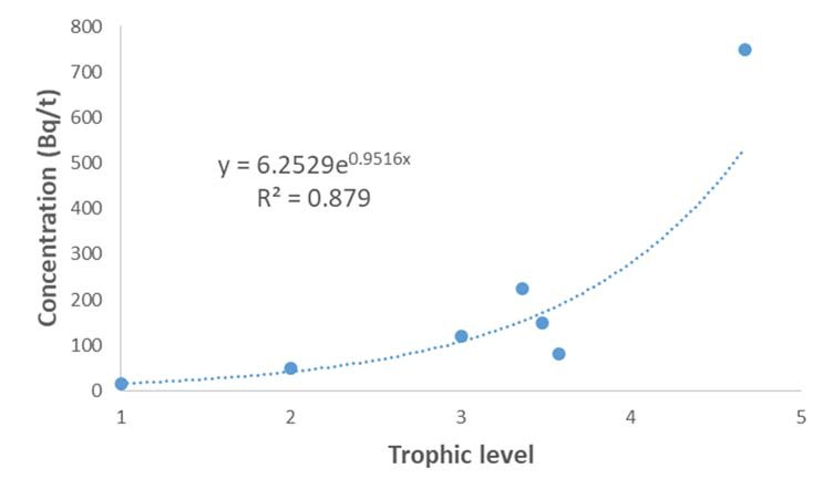
Figure 2. Relation between concentration in functional groups and trophic level used to estimate the direct adsorption rate.
