13 Network analysis
EwE links concepts developed by theoretical ecologists, especially the network analysis theory of Ulanowicz[1], with those used by biologists involved with fisheries, aquaculture and farming systems research. The Network analysis component of Ecopath is included as a plugin (Ecopath > Output > Tools > Network analysis).
The output forms included in the plug-in include: Trophic level decomposition, Flows and biomasses, Primary production required, Mixed trophic impact, Ascendancy, Flow from detritus, Cycles and pathways, Network analysis indices in Ecosim.
Trophic level decomposition
In addition to the routine for calculation of fractional trophic levels, a routine is included in Ecopath which aggregates the entire system into discrete trophic levels sensu Lindeman. This routine, based on an approach suggested by Ulanowicz[2] (1995), reverses the routine for calculation of fractional trophic levels. Thus, for the example when a group obtains 40% of its food as a herbivore and 60% as a first-order carnivore, the corresponding fractions of the flow through the group are attributed to the herbivore level and the first consumer level.
The results of this analysis are presented in the Relative flows table under the Trophic level decomposition node (these are proportions adding up to 1). These proportions are converted to absolute amounts, presented in the Absolute flows table (t km-2 year-1 or grams of carbon m-2 year-1), thus enabling the flows to be aggregated by trophic level and summarized in different ways.
Flows from detritus to the different model groups are calculated when you select the Flow from detritus menu item.
Transfer efficiency
Based on the trophic aggregation tables, the transfer efficiencies between successive discrete trophic levels can be calculated as the ratio between the sum of the exports from a given trophic level, plus the flow that is transferred from trophic level to the next, and the throughput on the trophic level. This is presented in a table with transfer efficiencies (%) by trophic levels.
Flows and biomasses
The absolute flows calculated in the Trophic level decomposition and Flow from detritus analyses can be aggregated to produce useful summaries by trophic level.
Primary production required
For terrestrial systems, it has been shown by Vitousek et al.[3] based on a detailed analysis of agriculture, industry and other activities, that nearly 40% of potential net primary production is used directly or indirectly by these activities. Comparable estimates for aquatic systems were not available until recently, though a rough estimate, of 2% was presented in the same publication. This figure, much lower than that for terrestrial systems, was based on the assumptions that an "average fish" feeds two trophic levels above the primary producers, and has been since revised upward.[4] The crudeness of Vitousek et al.’s approach for the aquatic systems was due mainly to lack of information on marine food webs, especially on the trophic positions of the various organisms harvested by humans. Models of trophic interactions may however help overcome this situation, and an alternative approach, based on network analysis, may be suggested for quantification of the primary productivity required to sustain harvest by humans (or by analogy by any other group that extracts production from an ecosystem).
To estimate the primary production required (PPR)[5] to sustain the catches and the consumption by the trophic groups in an ecosystem, the following procedure has been implemented in Ecopath: First, all cycles are removed from the diet compositions, and all paths in the flow network are identified using the method suggested by Ulanowicz.[6] For each path, the flows are then raised to primary production equivalents using the product of the catch, the consumption/production ratio of each path element times the proportion the next element of the path contributes to the diet of the given path element. For a simple path from trophic level (TL) I (primary producers and detritus), over TL II and III, and on to the fishery,
[latex]TL_I \xrightarrow{Q_{II}} TL_{II} \xrightarrow{Q_{III}} TL_{III} \xrightarrow{Q_{IV}} \text{Fishery}\tag{1}[/latex]
the primary production (or detritus) equivalents, PPR, corresponding to the catch of Y is:
[latex]PPR_C=Y \cdot \frac{Q_{III}}{Y} \cdot \frac{Q_{II}}{Q_{III}} = Q_{II} \tag{2}[/latex]
For the general (and more realistic) case where the pathways include branching the PPR corresponding to a catch Y of a given group can be quantified by summing over all pathways leading to the given group the PPR’s
[latex]PPR_C=\sum\limits_{\text{Paths}}(Y \cdot \prod\limits_{\text{Pred,prey}}\frac{Q_{\text{Pred}}}{P_{\text{Pred}}} \cdot DC'_{\text{Pred,prey}} ) \tag{3}[/latex]
where P is production, Q consumption, and DC’ is the diet composition for each predator/prey constellation in each path (with cycles removed from the diet compositions).
Further, the PPR for sustaining the consumption of each trophic group in a system can be estimated from the same equation as above by substituting the catch, Y, with the production term, P, calculated as the production/biomass ration, P/B, times the biomass, B.
PPR should actually be interpreted as flow from TL I as it includes primary production as well as detritus uptake. The denominator, PP, thus actually includes all "new" flow to the detritus groups, i.e. flow from primary producers and import of detritus.
The PPR is closely related to the "emergy" concept of H. T. Odum,[7] and is proportional to the "ecological footprint" of Wackernagel and Rees.[8]
Mixed trophic impacts
Leontief [9] developed a method to assess the direct and indirect interactions in the economy of the USA, using what has since been called the "Leontief matrix". This approach was introduced to ecology by Hannon[10] and Hannon and Joiris.[11] Using this, it becomes possible to evaluate the potential effect that a small change in the biomass of a group may have on the biomass of the other groups in a system. Ulanowicz and Puccia[12] developed a similar approach, and a routine based on their method has been implemented in the Ecopath system. The "mixed trophic impact" (MTI) for living groups is calculated by constructing an n x n matrix, where the i,jth element representing the interaction between the impacting group i and the impacted group j is
[latex]MTI_{i,j}=DC_{i,j} - FC_{ji} \tag{4}[/latex]
where DCi,j is the diet composition term expressing how much j contributes to the diet of i, and FCj,i is a host composition term giving the proportion of the predation on j that is due to i as a predator. When calculating the host compositions the fishing fleets are included as ‘predators’.
For detritus groups the DCi,j terms are set to 0. For each fishing fleet a "diet composition" is calculated representing how much each group contributes to the catches, while the host composition term as mentioned above includes both predation and catches.
The diagonal elements of the MTI are further increased by 1, i.e.,
[latex]MTI_{i,i}= MTI_{i,i}+1 \tag{5}[/latex]
The matrix is inversed using a standard matrix inversion routine.
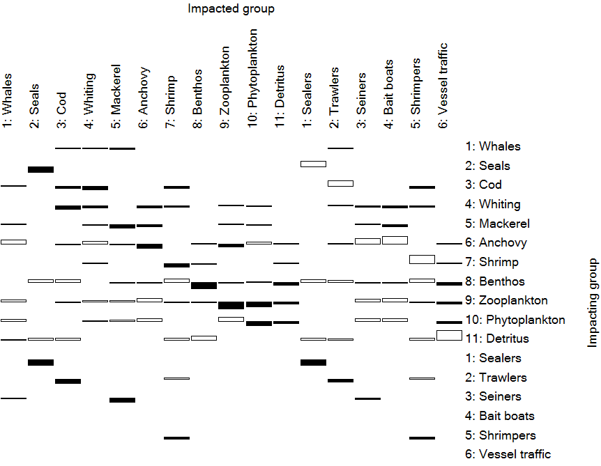
Figure 1. Mixed trophic impacts for Anchovy Bay showing the combined direct and indirect trophic impacts that an infinitesimal increase of any of the groups in the rows (to the right) is predicted to have on the groups in the columns (on top). The open bars pointing upwards indicate positive impacts, while the filled bars pointing downwards show negative impacts. The bars should not be interpreted in an absolute sense: the impacts are relative, but comparable between groups.
Note in Figure 1 that most groups have a negative impact on themselves, interpreted here as reflecting increased within-group competition for resources. Exceptions exist; thus, if a group cannibalizes itself (0-order cycle), the impact of a group on itself may be positive. In figure 1 the impact of whales on whales is negligible indicating that whales very far from their carrying capacity in the model base year.
The mixed trophic impact routine can also be regarded as a form of "ordinary" sensitivity analysis.[13] In this system, it can be concluded, e.g., that the impact of the bathypelagics on any other group is negligible: these fishes are too scarce to have any quantitative impacts. This can be seen to indicate that one need not allocate much effort in refining one’s parameter estimates for this group; it may be better to concentrate on other groups.
One should regard the mixed trophic impact routine as a tool for indicating the possible impact of direct and indirect interactions (including competition) in a steady-state system, not as an instrument for making predictions of what will happen in the future if certain interaction terms are changed. The major reason for this is that changes in abundance may lead to changes in diet compositions, and this cannot be accommodated with the mixed trophic impact analysis.
Ascendancy
"Ascendency" is a measure of the average mutual information in a system, scaled by system throughput, and is derived from information theory.[14] If one knows the location of a unit of energy the uncertainty about where it will next flow to is reduced by an amount known as the average mutual information’,
[latex]I= \sum\limits_{i=1,j=1}^n f_{}ij Q_i \log(f_{ij}/\sum\limits_{k=1}^n) f_{kj}Q_k \tag{6}[/latex]
where, if Tij is a measure of the energy flow from j to i, fij is the fraction of the total flow from j that is represented by Tij, or,
[latex]f_{ij}=T_{ij}/\sum\limits_{k=1}^n T_{kj} \tag{7}[/latex]
Qi is the probability that a unit of energy passes through i, or
[latex]Q_i=\sum\limits_{k=1}^n / \sum\limits_{l=1,m=1}^n T_{lm} \tag{8}[/latex]
Qi is a probability and is scaled by multiplication with the total throughput of the system, T, where
[latex]T=\sum\limits_{i=1,j=1}^n T_{i,j} \tag{9}[/latex]
Further
[latex]A=T \cdot I \tag{10}[/latex]
where A is called "ascendency". The ascendency is symmetrical and will have the same value whether calculated from input or output.
There is an upper limit for the size of the ascendency. This upper limit is called the "development capacity" and is estimated from
[latex]C = H \cdot T \tag{11}[/latex]
where H is called the ‘statistical entropy’, and is estimated from
[latex]H=\sum\limits_{i=1}^n Q_i \log Q_i \tag{12}[/latex]
The difference between the capacity and the ascendency is called "system overhead". The overheads provide limits on how much the ascendency can increase and reflect the system's "strength in reserve" from which it can draw to meet unexpected perturbations.[15] As an example, the part of the ascendency that is due to imports, A0, can increase at the expense of the overheads due to imports, Q0. This can be done by either diminishing the imports or by importing from a few major sources only. The first solution would imply that the system should starve, while the latter would render the system more dependent on a few sources of imports. The system thus does not benefit from reducing Q0 below a certain system-specific critical level (Ulanowicz and Norden, 1990).
The ascendency, overheads and capacity can all be split into contributions from imports, internal flow, exports and dissipation (respiration). These contributions are additive.
The unit for these measures is "flowbits", or the product of flow (e.g., t km-2 year-1) and bits. Here the "bit" is an information unit, corresponding to the amount of uncertainty associated with a single binary decision.
The overheads on imports and internal flows (redundancy) may be seen as a measure of system stability sensu Odum, and the ascendency / system throughput ratio as a measure of information, as included in Odum’s attributes of ecosystem maturity. For a study of ecosystem maturity using Ecopath see Christensen 1995.[16]
Flow from detritus
The Trophic level decomposition analysis calculated the fractions of the flow from each trophic level through each model group. The Flow from detritus analysis is equivalent, but calculates the flow from detritus through each group and converts it to absolute flows (t km-2 year-1).
Cycles and pathways
A routine based on an approach suggested by Ulanowicz[17] has been implemented to describe the numerous cycles and pathways that are implied by the food web representing an ecosystem.[18]
Each routine below has two forms: Pathway and Summary of pathways. The summary routine counts the number of all pathways leading from the prey to the selected consumer. The mean path length will be calculated and displayed on the form. It is calculated as the total number of trophic links divided by the number of pathways.
Consumer <- TL1
This routine lists all pathways leading from all groups on Trophic Level I (primary producers and detritus) to any selected consumer. A list of all consumers in the system will be displayed, and one can select from this. The program then searches through the diet compositions, finds all the pathways from the primary producers to the specified consumer, and then presents these pathways. Further, a summary presents the total number of pathways and the mean length of the pathways (under the Summary of pathways menu item). The latter is calculated as the total number of trophic links divided by the number of pathways.
Consumer <- prey <- TL1
This routine lists all pathways leading from all groups on Trophic Level I (primary producers and detritus) to any selected consumer via a selected prey. A pull-down list of all consumers in the system will be displayed after the heading “Pathways leading to:”. Select the consumer of interest from this list then choose a specific prey from the right-hand pull-down list. The program searches through the diet compositions, finds all the pathways from the primary producers, via the selected prey, to the specified consumer, and then presents the pathways. A summary presents the total number of pathways and the mean length of the pathways (under the Summary of pathways menu item).
Top predator <- prey
Here, one enters a prey group, and the program will find all pathways leading from this prey to all top predators. A summary presents the total number of pathways and the mean length of the pathways (under the Summary of pathways menu item).
Cycles (living)
The routine identifies all cycles in the system excluding detritus and displays these, in ascending order, starting with "zero order" cycles ("cannibalism"). In addition, the total number and the mean length of the cycles will be displayed.
Cycles (all)
The routine identifies all cycles in the system and displays these, in ascending order, starting with "zero order" cycles ("cannibalism"). In addition, the total number and the mean length of the cycles will be displayed.
Cycling and path length
The "cycling index" is the fraction of an ecosystem's throughput that is recycled. This index, developed by Finn[19] (1976), is expressed here as a percentage, and quantifies one of Odum's[20] 24 properties of system maturity.[21] Recent work shows this index to strongly correlate with system maturity, resilience and stability.
In addition to Finn's cycling index, Ecopath includes a slightly modified "predatory cycling index", computed after cycles involving detritus groups have been removed.
The path length is defined as the average number of groups that an inflow or outflow passes through.[22]. It is calculated as
Path length = Total System Throughput / (∑Export + ∑Respiration)
As diversity of flows and recycling is expected to increase with maturity, so is the path length. The effects of changes in the ecosystem on the network analysis indices (such as total systems throughput, Finn and predatory cycling indices, ascendency, overhead and their breakdown into various components) can then be plotted over time and compared for various scenarios of Ecosim.
Attribution: This chapter is in part adapted from the unpublished EwE User Guide: Christensen V, C Walters, D Pauly, R Forrest. Ecopath with Ecosim. User Guide. November 2008.
- Ulanowicz, R. E., 1986. Growth and Development: Ecosystem Phenomenology. Springer Verlag (reprinted by iUniverse, 2000), New York. 203 pp. ↵
- Ulanowicz, R. E., 1995. Ecosystem Trophic Foundations: Lindeman Exonerata. In: Chapter 21 p. 549-560 In: B.C. Patten and S.E. Jørgensen (eds.) Complex ecology: the part-whole relation in ecosystems, Englewood Cliffs, Prentice Hall. ↵
- Vitousek, P. M., Ehrlich, P. R., and Ehrlich, A. H. 1986. Human appropriation of the products of photosynthesis. Bioscience, 36:368-373. ↵
- Pauly, D., and Christensen, V. 1995. Primary production required to sustain global fisheries. Nature, 374(6519):255-257 [Erratum in Nature, 376: 279]. ↵
- Christensen, V., and Pauly, D., 1993. Flow characteristics of aquatic ecosystems. In: Trophic Models of Aquatic Ecosystems. pp. 338-352, Ed. by V. Christensen and D. Pauly, ICLARM Conference Proceedings 26, Manila ↵
- Ulanowicz, R. E., 1995. Ecosystem Trophic Foundations: Lindeman Exonerata. In: Chapter 21 p. 549-560 In: B.C. Patten and S.E. Jørgensen (eds.) Complex ecology: the part-whole relation in ecosystems, Englewood Cliffs, Prentice Hall. ↵
- Odum, H. T. 1988. Self-organization, transformity and information. Science, 242:1132-1139. ↵
- Wackernagel, M., and Rees, W., 1996. Our ecological footprint: reducing the human impact on the Earth. In: New Society Publishers. Gabriela Island. 160 p. ↵
- Leontief, W. W., 1951. The Structure of the U.S. Economy. Oxford University Press, New York. ↵
- Hannon, B. 1973. The structure of ecosystems. J. Theor. Biol., 41:535-546. ↵
- Hannon, B., and Joiris, C. 1989. A seasonal analysis of the southern North Sea ecosystem. Ecology, 70(6):1916-1934. ↵
- Ulanowicz, R. E., and Puccia, C. J. 1990. Mixed trophic impacts in ecosystems. Coenoses, 5:7-16. ↵
- Majkowski, J., 1982. Usefulness and applicability of sensitivity analysis in a multispecies approach to fisheries management. In: Theory and management of tropical fisheries. ICLARM Conf. Proc. 9. pp. 149- 165, Ed. by D. Pauly and G. I. Murphy ↵
- see Ulanowicz, R. E., and Norden, J. S. 1990. Symmetrical overhead in flow and networks. Int. J. Systems Sci., 21(2):429-437 ↵
- Ulanowicz, 1986. op. cit. ↵
- Christensen, V. 1995. Ecosystem maturity - towards quantification. Ecological Modelling, 77(1):3-32. ↵
- Ulanowicz. 1986. op.cit. ↵
- For a further description see Ulanowicz, 1986, his examples 4.4 and 4.5, page 65f.) ↵
- Finn, J. T. 1976. Measures of ecosystem structure and function derived from analysis of flows. J. Theor. Biol., 56:363-380. ↵
- Odum, 1969. op. cit. ↵
- Christensen 1995. op. cit. ↵
- Finn JT. 1980. Flow analysis of models of the Hubbard Brook ecosystem. Ecology 6: 562-571. ↵
