38 Fleet effort dynamics

There are three ways to specify temporal changes in fishing fleet sizes and fishing effort:

1. By sketching temporal patterns of effort in the model run interface;
2. By entering annual patterns via reference CSV files along with historical ecological response data; and
3. By treating dynamics of fleet sizes and resulting fishing effort as unregulated and subject to fisher investment and operating decisions (“bionomic” dynamics, fishers as dynamic predators).

To facilitate exploration of alternative harvest regulation policies, the Ecosim default options are (1) or (2).  However, you can invoke the fleet/effort dynamics model where effort is estimated, rather than input, by checking Ecosim > Input > Ecosim parameters > Fleet effort dynamics. Input parameters must then be set on the Ecosim > Input > Fleet size dynamics form.

When the fleet/effort response option is invoked, Ecosim  starts each by erasing all previously entered time patterns for fishing efforts and fishing rates, and replaces these with simulated values generated as each simulation proceeds. The fleet/effort dynamics simulation model uses the idea that there are two time scales of fisher response:

1. A short time response of fishing effort to potential income from fishing, within the constraints imposed by current fleet size, and
2. A longer time investment/depreciation “population dynamics” for capital capacity to fish (fleet size, vessel characteristics).

These response scales are represented in Ecosim by two “state variables” for each gear type g.

Fast time response model

E_g,t is the current amount of effort (active, searching gear, scaled to 1.0 at the Ecopath base fishing mortality rates), and K_g,t is the maximum possible effort (E_g,t < K_g,t).

At each time step, a mean income per effort index I_g,t is calculated as

[latex]I_{g,t}=\sum_i q_{g,i} B_i P_{g,i} \tag{1}[/latex]

where i = ecological species or biomass group, q_g,i is the catchability coefficient (possibly dependent on B_i) for species i by gear g, and P_g,i is the market price obtained per biomass of i by gear g fishers.  Also, mean fleet profit rates PR_g,t for fishing are calculated thus:

[latex]PR_{g,t}=I_{g,t}-c_g \tag{2}[/latex]

where c_g is the cost of a unit of fishing effort for gear g (cost and price factors are entered via the Definition of fleets and Market price forms). For each time step, the “fast” effort response for the next (monthly) time step is predicted by a sigmoid function of income per effort and current fleet capacity:

[latex]E_{g,t+1}=\frac{K_{g,t}I^p_{g,t}}{I^p_{hg}+I^p_{g,t}} \tag{3}[/latex]

Here, I_hg and p are fleet-specific response parameters. I_hg is the income level needed for half maximum effort to be deployed and p is a “heterogeneity” parameter for fishers: high p values imply all fishers “see” income opportunity similarly (start or quit at similar income values), while low p values imply fishers “turn on” their effort over a wide range of mean incomes (start or quit over a wide range of average incomes), as shown in Figure 1.

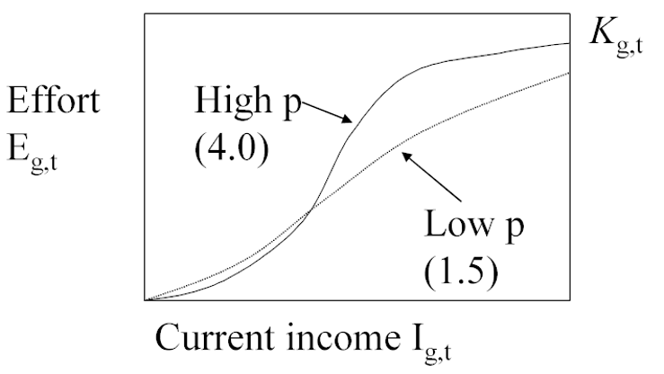
Figure 1. Effect of the “heterogeneity” parameter, p, on effort/income function.

Slow time response model

For each fleet, slow effort responses are modelled as changes in fleet capacity (K_g,t), which is a function of the capital depreciation rate ρ_g, the capital growth rate r_g,t and profit PR_g,t. The capital growth rate is calculated via a growth factor gf_g,t, i.e.,

[latex]gf_{g,t+1}=\frac{K_{g,t}(r_{g,t}+\rho_g)}{PR_{g,t}} \tag{4}[/latex]

where Kg,1, ρg and rg,1 are set by the user. The annual capacity Kg,t is then updated as

[latex]K_{g,t+1}=K_{g,t}(1-\rho_g)+gf_{g,t}PR_{g,t+1} \tag{5}[/latex]