Tutorial: Group info
Learning Objectives
- Introduce the Ecosim Group Info parameters
- Get an idea of what they do
- See how their settings may impact results
- Get an idea of when to change these parameters
In this tutorial, we once again head to Anchovy Bay – If you don’t have the model at hand, you can download it from this link.
The purpose of this tutorial is to take you through the parameters on the Ecosim > Input > Group info page, explain what they are, and play a bit with them.
Max rel. P/B
This parameter sets a cap for primary producers for how much P/B can relatively increase from the Ecopath level. It is rarely used as P/B for producers seldom changes much in Ecosim. Invoke if you have a primary producer where you can see on the Ecosim > Output > Ecosim group plots that its P/B reaches the ceiling specified by the Max rel. P/B setting.
See also the User Guide system productivity chapter.
Example 1: Max rel. P/B
If you want to have a go, you can make a forcing function, go to Ecosim > Input > Forcing functions, and add a forcing function if you don’t have one, then sketch an increased level of around 3 for the function. Go to Ecosim > Input > Forcing Function > Apply forcing (producer) and apply the function to phytoplankton by clicking the field by the group, then applying the function of the pop-up form.
Note that a 3 x increase in primary production is highly unlikely, this is just for demonstration.
Run the model with the default Max rel. P/B setting (2), and you’ll probably see that the model has become unstable, that phytoplankton fluctuates wildly and overall have declined while zooplankton, also unstable, have increased.
Then set Max rel. P/B to 5, and run again. You’ll probably see that the model still is unstable but phytoplankton now increases. They can increase production more before zooplankton builds up.
Again, this is a highly unrealistic scenario, just for demonstration.
Max rel. feeding time
This parameter set how much the feeding time can increase (relative to the Ecopath baseline) if a predator becomes more abundant and/or its prey becomes more sparse. The parameter only takes effect if the feeding time adjustment rate is > 0.
Feeding time adjust rate [0,1]
The feeding time adjustment is used to model compensatory growth. Setting this parameter (> 0) allows Ecosim to vary Q/B as a function of the group biomass – organisms will seek to maintain Ecopath base Q/B by varying relative feeding time
The key question is: how does a species react when its prey abundance change? Will it spend more time feeding to maintain the consumption rate when prey are sparse – being exposed to predation for longer – or does it have a fixed diurnal pattern, so that less prey means lower consumption?
Many species indeed have fixed diurnal runs and we advise to keep feeding time constant for all groups apart from marine mammals, birds and maybe top predators. Also for very young stages of multi-stanza groups.
We can examine what the setting does for cod in the Anchovy Bay model. Run your model with default settings and you’ll probably see that cod declines because of the increase in trawler effort. Set Ecosim to display multiple runs at Ecosim > Output > Run Ecosim > Show multiple runs. Examine the Ecosim > Output > Ecosim group plots for cod, note how feeding time changes and how much Q/B (Consumption/biomass) increases – fewer cod means more food each of them, that’s why the cod doesn’t just decline in a straight line, there is compensation.
Next, set the Ecosim < Input < Group info > Feeding time adjust rate to 0 (for no change in feeding time). Run again, and see what happens.
Example 2: Feeding time adjust rate
Figure 1 shows some results for illustration. You’ll notice that with the default setting (Feeding time adjust rate of 0.5) the cod declines strongly, but there is some compensation as can be seen from the top right plot with shows Q/B increase from ~2.6 to ~4 year-1. When feeding rate is kept constant (Feeding time adjust rate of 0.0, center right plot) there is more compensation as seen from Q/B increasing to ~5 year-1, and the cod decline is less drastic.
The figures for comparison also shows the effect of setting the handling time parameter, QBmax/QBo, to 1.2, see the corresponding section later in this chapter. Note that here this parameter leads to even less compensation in consumption rate as biomass declines (lower right plot).

Figure 1. Ecosim trajectories (left) for cod in the Anchovy Bay model under three different configurations along with Q/B rates for cod for the same settings, which are Feeding time adjusmt rateat 0.5 (default, top right figure) and 0 (constant feeding time, center right figure), Qmax/Qo reduced to 1.2 (all other settings at default values, lower right figure).
Fraction of other mortality sens(itive) to changes in feeding time
This parameter decides what happens to the other mortality when feeding time changes. The general assumption is that if feeding time increases so will the other mortality – the underlying assumption being that the other mortality may be due to predators not included in the model. There may not be any such predators, so you have the option to set the parameter to 0.
We can check what happens in Anchovy Bay. Run your model with default settings, and check the results (Ecosim > Output > Ecosim group plots) for shrimp. Next set the Fraction of other mortality sens. to changes in feeding time to 0, and run again. Compare the results.
Example 3: Fraction of other mortality sens. to changes in feeding time
Figure 2 shows the effect of the default setting for the Fraction of other mortality sens. to changes in feeding time (1) along with when the parameter is set to 0. When cod and whiting declines in the model, the predation rate on shrimp declines as well, but with default setting (right side top figure) the other mortality for shrimp increases as shrimp spends more time fitting as their population grows. When the impact on other mortality is turned off (right side lower figure) the other mortality stays constant and the increase in shrimp biomass is greater than with the default settings (left hand side figure).
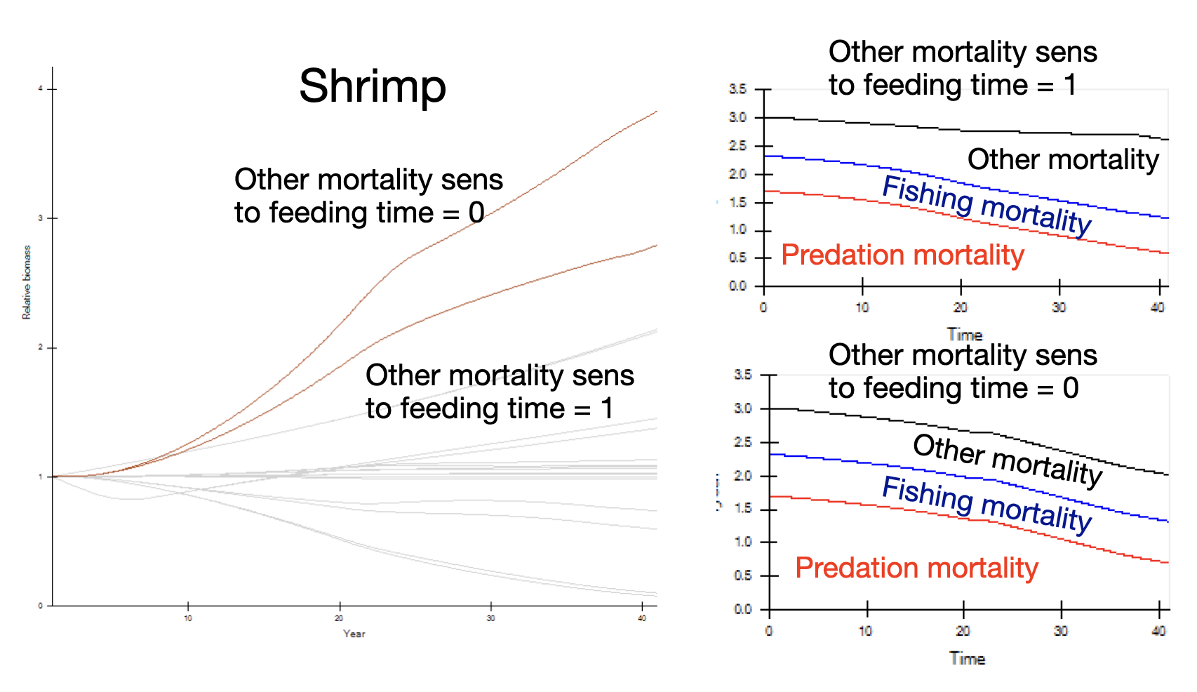
Figure 2. Effect of predator effect on feeding time for shrimp in the Anchovy Bay model.
Predator effect on feeding time [0,1]
Predators can be scary, it’s dangerous to be a fish. If there are predators around, prey fish tend to change behaviour. It’s better to not eat than be eaten, so predators can limit prey’s consumption rate. We can include this effect through the Predator effect on feeding time parameter.
In your Anchovy Bay model, make a run, check out the results for shrimps (Ecosim > Output > Ecosim group plots) . Next set the Predator effect on feeding time to 1, and run again. Compare the results.
Example 4: Predator effect on feeding time
Figure 3 shows the result of Predator effect on feeding time settings. With the default setting (0) predators do not impact the feeding time (top centre plot in Figure 3). The feeding time for shrimp here increase from 1 to >4 as there becomes more and more shrimp competing for their food resources. The total mortality of shrimp decreases due to declining predation mortality (Figure 1, top right).
Running the model again with Predator effect on feeding time on (set to 1), there are some changes (Figure 1, lower centre and right plots). As the predation mortality on shrimp decreases, the shrimp feeding time increases, but much less than in the initial run. By the end, feeding time has just doubled (vs. >4 times in the first run) and shrimp biomass have increased much less. In essence, merely by predators being around they limit how much shrimp feeding time increases, and this constrains increase in shrimp biomass. Indeed, the lower right plot shows that the total mortality for shrimp increases toward the end of the run, rather than decreases as in the top right plot.
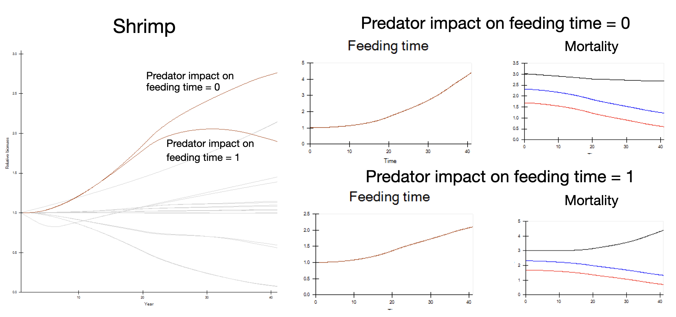
Figure 3. Effect of the Predator impact on feeding time parameter for shrimp in Anchovy Bay.
Density-dep. catchability, Qmax/Qo [>=1]
Is catch per unit effort (CPUE) proportional to stock biomass? Well if it is, no worries, you can leave this parameter at its default value. Density-dependent catchability is used where catchability can increase relative to the Ecopath baseline. This could for instance be for pelagic species that are caught with purse seines. It may take at little longer to find a school of pelagics when abundance go down but the CPUE probably declines less than the stock. For demersal species the same effect can happen if there’s range contraction when abundance declines, that can lead to CPUE remain high even if stock declines. Let’s explore this in Anchovy Bay.
In your model, go to Ecosim > Input > Fishing Effort, click on fleet 3 Seiners, and Set to value of 2 to double the effort of seiners (which catch mackerel). Run your model and set Ecosim to display multiple runs at Ecosim > Output > Run Ecosim > Show multiple runs. Next, go to Ecosim > Input > Group info and set the Density-dep. catchability, Qmax/Qo parameter for mackerel to 2, repeat with 4, 8, 16, … What’s the impact of this on mackerel?
Density-dependent catchability parameters are discussed in the User Guide’s chapter on catchability.
Example 5: Density-dep. catchability, Qmax/Qo [>=1]
Figure 4 shows how mackerel reacted to a doubling in the effort of seiners when the Density-dep. catchability, Qmax/Qo was increased in steps from 1 to 128. The top insert shows the mackerel fishing mortality (F) with the default setting (1) and with a setting of 128. At the default setting the F is constant through the run, with higher Qmax/Qo values F increases when the biomass is reduced, i.e. CPUE is not proportional to effort.

Figure 4. Impact of density dependent catchability for mackerel in Anchovy Bay. The Qmax/Qo parameter setting is indicated in the black markers.
QBmax/QBo (for handling time) [>1]
The handling time parameter limits consumption of prey at high prey densities, but can have a destabilizing effect at low densities. See Figure 1 for an example.
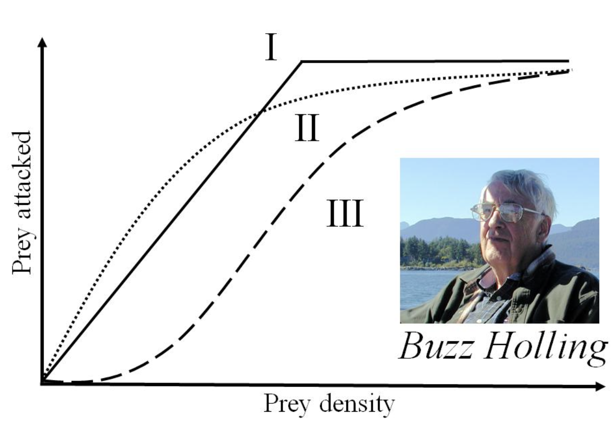
Figure 5. Functional responses indicating number of prey attacked as a function of prey density. These functional responses were defined and developed by CS Holling[1] [2]. Type 1 indicates a linear relationship and might, e.g., be used for a spider web, Type 2 is with handling time included (Disk Equation) and type III is with switching.
Switching power parameter [0,2]
Example 6: Switching power parameter
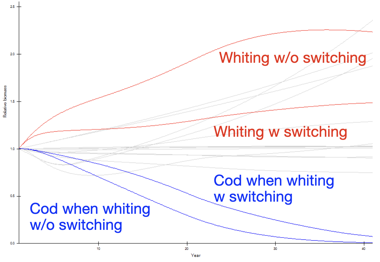
Figure 6. Output from runs with default settings and with the switching parameter for whiting set to 2.
- Holling, C.S. (1959a) The components of predation as revealed by a study of small-mammal predation of the European pine sawfly. The Canadian Entomologist 91, 293-320. https://doi.org/10.4039/Ent91293-5 ↵
- Holling, C.S. (1959b) Some characteristics of simple types of predation and parasitism. The Canadian Entomologist 91, 385–398. https://doi.org/10.4039/Ent91385-7 ↵
