Tutorial: Welcome to Anchovy Bay
Learning Objectives
By the end of this tutorial, participants will be able to:
- Initiate and Configure a Basic Ecopath Model: Create a new EwE project, define essential functional groups (including primary producers and detritus), and establish relevant fishing fleets for a given ecosystem.
- Parameterize an Ecopath Model with Diverse Data: Input ecological data, including biomass, production-to-biomass (P/B), consumption-to-biomass (Q/B) ratios, catch data, and diet compositions, using provided values and deriving estimates from external sources (e.g., FishBase, allometric relationships).
- Achieve and Interpret Ecopath Mass Balance: Understand the underlying principles of mass balance in Ecopath and utilize the software's tools to iterate towards a balanced model, critically evaluating the estimated ecotrophic efficiencies (EEs) and other output parameters.
- Perform Initial Model Diagnostics and Exploration: Generate and interpret basic Ecopath outputs, such as "Basic estimates" and "Mixed Trophic Impact," to gain preliminary insights into ecosystem structure and trophic interactions.
- Navigate the EwE Interface for Fundamental Operations: Use the Ecopath with Ecosim (EwE) software to create models, input data, access key diagnostic tools, and conduct simple exploratory changes to model parameters.
- Recognize Data Requirements and Acquisition Strategies: Identify the specific data types required for Ecopath modeling and understand various practical approaches for acquiring or estimating these data, acknowledging limitations and uncertainties when information is incomplete.

Figure 1. Simplified basemap of Anchovy Bay from a spatial ecosystem model.
Colour gradient indicates depth and the black dots harbours.
The purpose of this tutorial is to introduce you to the Ecopath with Ecosim (EwE) software, explore what data is required, give examples of where you can get such data, and go through the steps that typically are required when constructing a model.
We acknowledge that if you are new to the subject area, you will struggle with this tutorial, but we've built is so that it takes you through it step by step with explanations as you go along, and we expect that you, with a bit of effort, will be able to work your way through it. Please take it as an introduction, when we later introduce and describe all the bits and pieces in detail, you'll have a better idea of how they fit together when you've done this tutorial.
Introduction to Anchovy Bay
Anchovy Bay is a popular tourist attraction with its century-old fishing port. Fisheries have traditionally been the mainstay of the area, but catches have declined for decades and shifted from a focus on groundfish to being dominated by shrimp and pelagics.
In recent years, a whale-watching industry has developed linked with growing interest in eco-tourism and recovery of marine mammal populations after earlier periods of whaling and culling.
We will use Anchovy Bay as a "model ecosystem" throughout this textbook. Anchovy Bay is in many ways ideal for this as it is is well-studied – to the degree where we have excellent information about the resources in the bay, about how the environment has changed, and of how fisheries and other factors impacting the ecosystem have developed in recent history. The exercises will use variable amounts of information, starting simple (and thereby illustrating the impact of, e.g., missing important drivers) for gradually to include more and more data. This is to simplify the presentation and analysis, but also to illustrate that one can still work with incomplete information – even if it makes conclusions less reliable and leave more questions open for interpretation.
Build an ecosystem model
Anchovy Bay covers an area of 10,000 km2. For this exercise, we assume that it is rather isolated from other marine systems, and that the populations stay in the bay year-round.
We want to create a model of the bay in 1970, with the following 11 groups:
Whales, seals, cod, whiting, mackerel, anchovy, shrimp, benthos, zooplankton, phytoplankton, detritus. [Hint: make a spreadsheet with these group names in rows, you’ll need to do more calculations later]
Start by opening EwE6, select Menu > File > New model. Browse to your preferred file location, and enter a name for the model. For instance, “Anchovy Bay”. Now navigate on the Navigator (left panel) to Input data > Basic Input. The model will have one group, Detritus.
All models must have a detritus group, so we have entered it for you. Why? We need to be sure there is a group where we can send flows of excreted and egested material as well as dead organism. By default, they go to the detritus group.
On the Basic input form, select Define groups (also available from the menu on top: Ecopath > Define groups). Click Edit > Insert on the right side of the form that pops up. Continue clicking Insert till you have 11 groups; then enter the group names, i.e., Whales in first row, Seals in second, etc. [Hint: you can cut and paste the names in one go from Excel, using Ctrl-C Ctrl-V]. When you have entered all, define that phytoplankton is a primary producer by clicking the Producer check mark in the phytoplankton row. On the right panel, you may also want to click the Colors > Alternate all, to get a better distribution of group colors (more distinguishable in Ecosim). Click OK.
We also need to define the fishing fleets. Click Ecopath > Input > Fishery on the Navigator to the left. Then click Fleets, and then Define fleets above the spreadsheet (or go Menu >Ecopath >Define fleets). We want five fleets: sealers, trawlers, seiners, bait boats, and shrimpers. We can enter catches at Ecopath > Input > Fishery > Landings; unit has to be t km-2 year-1. The sealers caught 1,500 seals in 1970 with an average weight of 30 kg. The fisheries catches were 4,500 t of cod and 2,000 t of whiting for the trawlers, 4,000 t of mackerel and 12,000 t of anchovy for the seiners, 2,000 t of anchovy for the bait boats, and 5,000 t of shrimp for the shrimpers. Calculate catches using the appropriate unit (t km-2 year-1), and enter in EwE.
Units are important. We all make conversion errors occasionally. Be explicit and check your units (biomass t km-2, flows t km-2 year-1). Conversion errors are the most common cause of problems with this tutorial.
The off-vessel landing prices (Ecopath > Input > Fishery > Off-vessel price) are seals $6 kg-1; cod: $10 kg-1; whiting $6 kg-1; mackerel: $4 kg-1; anchovy from seiners $2 kg-1, and $3 kg-1 for bait boats. Shrimps are $20 kg-1. [While landings are in t, it is fine for now to enter landing prices in $/kg to avoid the extra ‘000s]. Prices are current prices (hence “are” instead of “were”) as we later will be using these for forward projections. If you lack catch or price information for your own models later, then search, check www.seaaroundus.org, ask around, or guess!
We now should enter the basic input parameters. Fortunately, there has been monitoring in the bay for decades, and we have some biomass survey estimates from 1970. The biomasses must be entered with the unit t km-2. Whales: 50 individuals with an average weight of 16,000 kg. Seals: 20,300 individuals with an average weight of 30 kg. Cod: 30,000 t. Whiting 18,000 t. Mackerel: 12,000 t. Anchovy: 70,000 t. Shrimp: 0.8 t km-2. Zooplankton: 14.8 t km-2, detritus 10 t km-2.
Next are production/biomass (P/B) ratios, which with certain assumptions (that we won’t worry about now) correspond to the total mortality, Z. The P/B are annual rates, so the unit is year-1. We often can get Z from assessments, or, alternatively, we have Z = F + M (i.e. we can estimate total mortality as the sum of fishing mortality, F and natural (predation) mortality, M). So, if we have the catch (C) and the biomass (B), we can estimate F = C/B and add the total natural mortality, M, to get Z.
For fish, we can get estimates of M and Q/B from FishBase. On the FishBase landings page, search for the species, (Gadus morhua, Scomber scombrus, Engraulis encrasicolus), one by one. From the species info screen for each, go to Tools > Life-history tool, and extract the Q/B and M values for each. Estimate Z = F + M. For whiting (Merlangius merlangus), we have local estimates of P/B = 0.58 year-1 and Q/B = 3.1 year-1.
For estimating Z for exploited species, it is also an option to use an equation that was developed by Ray Beverton and Sidney Holt[1]. It is implemented in the life-history tool table in FishBase. It relies on estimates of length at first capture (Lc), average length in the catch (Lmean), and asymptotic length (Linf) to estimate Z. Try it for the three species here. Here are the lengths from the fishery in Anchovy Bay:
| Lc (cm) | Lmean (cm) | |
| Cod | 52 | 72 |
| Mackerel | 18.9 | 26 |
| Anchovy | 6.8 | 10 |
Compare the P/B = Z estimates from the two methods (and consider = decide what to use). Maybe even try both estimates in Ecopath?
There is a close relationship between size and P/B; the bigger animals are, the lower the P/B. Here we have: Whales: P/B = 0.05 year-1; seals: get F from catch, and M is 0.09 year-1; shrimp P/B = 3 year-1; benthos P/B = 3 year-1; zooplankton: it is mainly small Acartia-sized plankton, with P/B = 35 year-1.
We can get P/B for many invertebrates from Tom Brey’s work (but don’t need to for this tutorial). Check out: http://www.thomas-brey.de/science/virtualhandbook/. There is a neat collection of empirical relationships and conversion factors. Also check SeaLifeBase.
Consumption/biomass (Q/B) ratios for the non-fish groups: for whales use 9 year-1, and for seals 15 year-1. For the invertebrates enter a P/Q ratio of 0.25 instead of entering a Q/B.
So, why enter P/Q instead of Q/B? When P/Q is an input, Ecopath will estimate Q/B = (P/B)/(P/Q). This makes it explicit that we haven't bothered to find a Q/B, but instead use the reasonable assumption that Q/B = 4 x P/B. We know that organisms only convert a fraction of their energy intake to production. For fish that fraction typically is 0.1-0.3, generally it relates to size where smaller organisms convert more efficiently than larger.
Finally, there is phytoplankton. We can often get primary production estimates from SeaWiFS satellite data. Here we have PP = 240 gC m-2 year-1. The conversion factor from gC to gWW is 9, so the total production, P, is 9 * 240 t km-2 year-1. You can set P/B to 120 year-1, and calculate B. The 120 year-1 is a guess, assuming that phytoplankton divides once per day in the productive part of the year (so less than 360/year), and is not very important as only the production, P = P/B * B is actually used in calculations. (Very high P/B values may, however, make Ecospace runs dizzy).
Next parameter is Ecotrophic Efficiency (EE), this is the part of the production that is used in the system (or rather, for which the model explains the fate of the production). In this model, we are missing a biomass estimate for benthos. We do not explain much of the mortality for this group, so we guess an EE = 0.6. For the other groups, we let Ecopath estimate the EEs, but bear in mind the definition of EE when you evaluate the estimated parameters.
In the Ecopath baseline year, the whale population had started to recover after whaling, but the seal population was still declining, so the Ecopath baseline model is not in steady state. We specify this on the Input data > Other production form by entering a biomass accumulation rate of 0.02 year-1 for whales, and –0.05 year-1 for seals.
Now it’s time for diets:
| # | Prey \ predator | 1 | 2 | 3 | 4 | 5 | 6 | 7 | 8 | 9 |
|---|---|---|---|---|---|---|---|---|---|---|
| 1 | Whales | 0 | 0 | 0 | 0 | 0 | 0 | 0 | 0 | 0 |
| 2 | Seals | 0 | 0 | 0 | 0 | 0 | 0 | 0 | 0 | 0 |
| 3 | Cod | 0.1 | 0.04 | 0 | 0.05 | 0 | 0 | 0 | 0 | 0 |
| 4 | Whiting | 0.1 | 0.05 | 0.05 | 0.05 | 0 | 0 | 0 | 0 | 0 |
| 5 | Mackerel | 0.2 | 0 | 0 | 0 | 0.05 | 0 | 0 | 0 | 0 |
| 6 | Anchovy | 0.5 | 0 | 0.1 | 0.45 | 0.5 | 0 | 0 | 0 | 0 |
| 7 | Shrimp | 0 | 0.01 | 0.01 | 0.01 | 0 | 0 | 0 | 0 | 0 |
| 8 | Benthos | 0.1 | 0.9 | 0.84 | 0.44 | 0 | 0 | 1 | 0.1 | 0 |
| 9 | Zooplankton | 0 | 0 | 0 | 0 | 0.45 | 1 | 0 | 0.1 | 0 |
| 10 | Phytoplankton | 0 | 0 | 0 | 0 | 0 | 0 | 0 | 0.1 | 0.9 |
| 11 | Detritus | 0 | 0 | 0 | 0 | 0 | 0 | 0 | 0.7 | 0.1 |
You should be able to cut-paste (Ctrl-C, Ctrl-V) from the spreadsheet above to the Ecopath diet screen. Or, you can download a spreadsheet with the diets from this link.
We now have the information that is needed to do mass-balance on this model. Select Output > Basic estimates, and check out the outcome. Save the model.
Try changing some of the input and see what happens. Don’t save afterwards.
Check out Network analysis (Ecopath > Output > Tools > Network analysis), especially, see the Mixed Trophic Impact plot
Go to Ecosim > Output > Run Ecosim > Run, and see what happens.
Explore the software.
Optionally and time permitting, here are some suggestions for things to try.
Network analysis: Mixed Trophic Impact
Network analysis is a research field often categorizing networks based on stock and flow properties. Output is often indicators of ecosystem state, performance and function. Explore the Network analysis available at Ecopath > Output > Tools > Network analysis for instance the Cycles and pathways, which identifies all cycles and pathways in the model. Or the Lindeman spline.
We'll focus though on a key network module in EwE. the Mixed Trophic Impact (MTI) analysis. MTI originates in the Nobel Prize work of Leontif[2] to assess demand-supply and direct and indirect interactions in the economy of the USA, using what has since been called the Leontief matrix or input-output model. In Ecopath network analysis, we have incorporated a derived approach developed by Ulanowicz and Puccia,[3] to quantify direct and indirect trophic impacts in an ecosystem.
You can find the MTI analysis at Ecopath > Output > Tools > Network analysis > Mixed Trophic Impacts > Mixed trophic impact plot where Options let you change Data to Colours and Plot > Fit to available area as options.
In the plot, red colours indicate negative competition effects and blue colours positive. The effects are relative and comparable across the ecosystems (fleets included). You can think of the effects as addressing the question: "if we were to change the biomass of the groups mentioned to the right of each row and infinitesimal[4] amount, what impact would this have on the groups listed above each column?"
Trace the simple connections between predators and prey to find direct impacts, notice how the diagonal indicates within-group competition.
Can you find any examples of what Sheila Heymans called "beneficial predation", i.e where a group preys on another group but still has a positive impact on the prey?[5]
- Why do seals not have any noticeable impact on any other groups? (apart from on Sealers)
- Why does mackerel have a positive impact on phytoplankton?
- Why do trawlers have a positive impact on shrimpers?
- Why does cod have a positive impact on bait boats?
While it's often straightforward to explain simple interactions, e.g., that a predator has a direct negative impact on it's prey, but a positive impact on the prey of the prey, the MTI excels at revealing indirect impacts driven by competition rather than direct food chain effects. It's really a neat analysis.
Ecosim: time dynamic simulation
We can now go straight to Ecosim now. Create a new Ecosim scenario, at the top-row menu select Ecosim > Create new scenario, and name it, e.g., "Ecosim try". Next, in the Navigator on the left, go Ecosim > Output > Run Ecosim, and click the Run button on the lower left. Ecosim will now run a multi-year simulation. Yes, there are default values that makes this possible.
We practice a "Model first, ask later" philosophy and find that getting you to run a model and ask questions, improve runs through model feedback, beats meticulous long-term model development before getting to get a sense of what matters through running the model.
The modelling philosophy thus also says: "When you start a new project, make a quick model the first week". Don't spend a year getting the data lined up before you start running your model. The initial model will make you focus on your research/policy questions from the onset as well as making it much clearer where you need to focus on your data accession. Also, it will tell you what matters less for the research/policy questions.
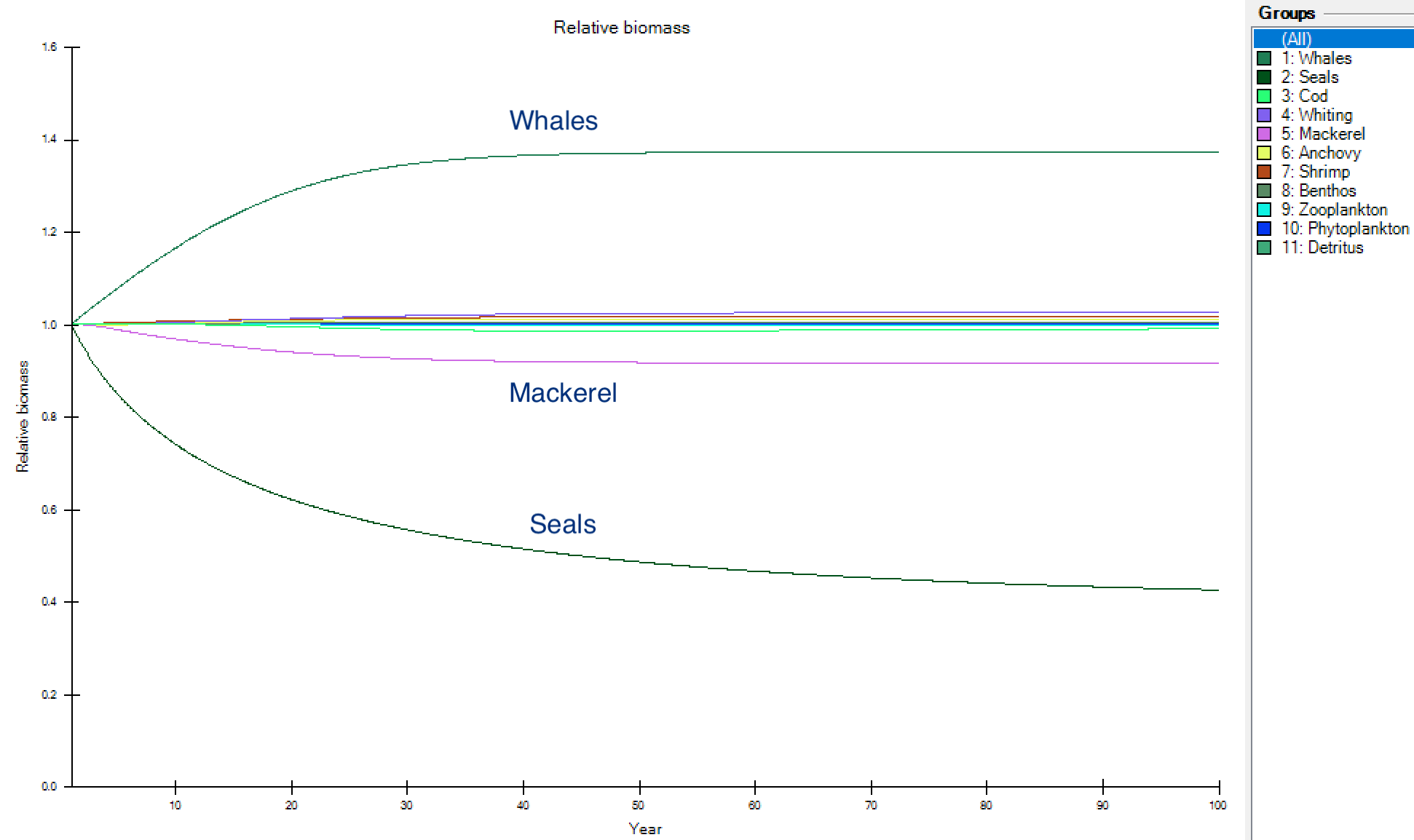
The first run probably looks like on the figure above[6].
- Why do whales increase?
- Why do seals decrease?
- Why do mackerel decrease?
These changes demonstrate that Ecopath is not a steady state model. When in Ecopath we include biomass accumulation (BA) for a group, we tell the model that the group wasn't in steady state in the base year. For Anchovy Bay, we have that whales were recovering from a long history of whaling (hence, a positive BA), and that the seals were declining because of over-exploitation (negative BA). Remember the second Ecopath Master Equation,
Production = predation + fishing mortality + net migration + biomass accumulation + other mortality
Note that there are cascading food web effects, why do mackerel decrease?
Also note that the increase/decrease for the whales and seals gradually moves toward an asymptotic level. Why? The answer to that question relates to the MTI we checked above. Remember how on the diagonal all impacts were negative? All groups compete with themselves for resources, that's not a surprise as all groups have a carrying capacity in the ecosystem: that's how much the resources they rely on can sustain. So, whales will gradually move toward that carrying capacity, and each seal will as their population decline get more food resources, leading to better growth and survival – in spite of continued seal exploitation.
So, we now have an Ecosim run, but is it credible? Certainly, the general pattern is OK, but how much would the whales and seals actually change if this was the real world?
To address that question,[7] remember the carrying capacity, a central aspect of all population modelling, which relates to density-dependence. The key, density-dependent parameter in Ecosim that captures carrying capacity is called the vulnerability multiplier. This parameter tells Ecosim how far from carrying capacity a predator is in the base Ecopath model relative to its carrying capacity: the default vulnerability multiplier of 2, tells Ecosim that if that predator was to grow to its carrying capacity it could at most increase the predation mortality it's causing on its prey with a factor or 2.
Whales and seals were both far from their carrying capacity in the base year, so we should expect their vulnerability multipliers to be higher than 2. Let's just guess that they could both increase the predation mortality that they are causing on their prey with an order of magnitude, that's setting their vulnerability multipliers to 10.
Let's try it. While you are on the Ecosim Run screen, click Show multiple runs above the plot. The go to Ecosim > Input > Vulnerabilities and click 1 in the heading row, enter 10 in the text box on the top right, click Apply next to the text book. It should now set the vulnerability multipliers to 10 for all whale prey groups. (You can also just enter 10 in each whale-prey cell, but the short cut is good to know). Now, do the same for seals by clicking on 2 in the heading row, etc.
Next go back to the Ecosim Run screen and run the model again. What happens now?
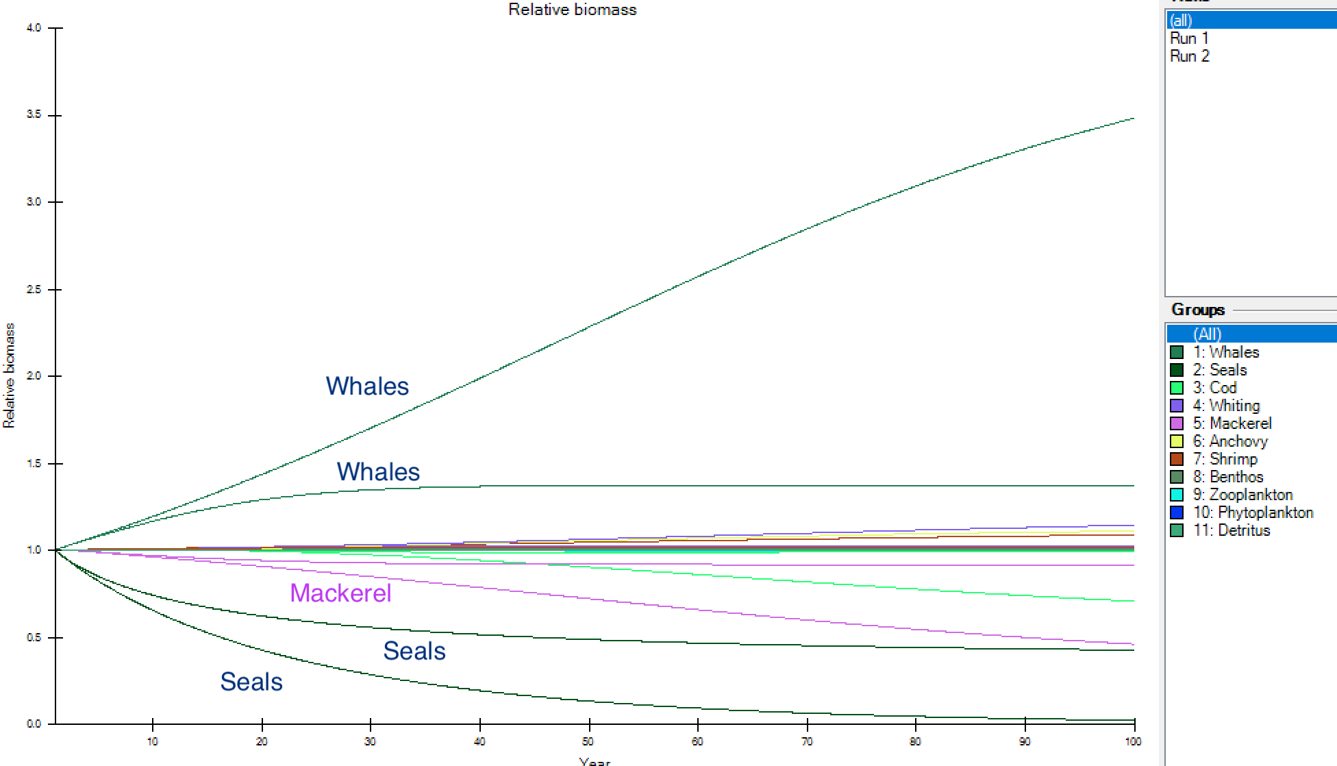
See the figure above, the whales now continue to grow, and the seals to decline. How do we then figure out how it should be? That's where time series come in. They can tell us how a group has reacted historically, and are essential for model fitting = getting a handle on the-one-parameter-in-Ecosim-that-rules-them-all, the vulnerability multipliers. But that's a tale for another day.
Feel free to explore your Anchovy Bay, remember it's "model first, ask later".
Media Attributions
- Ecospace > Input > Maps
- Original
- Original
- Beverton, R.J.H. and Holt, S.J. 1957. On the dynamics of exploited fish populations. Fisheries Investigations, 19, 1-533. ↵
- Leontief, W. W., 1951. The Structure of the U.S. Economy. Oxford University Press, New York. ↵
- Ulanowicz, R. E., and Puccia, C. J. 1990. Mixed trophic impacts in ecosystems. Coenoses, 5:7-16. ↵
- "infinitesimal" to indicate a small change that doesn't impact food availability noticeably. ↵
- Spoiler alert: check whales' or mackerel's MTI and diet ↵
- If not, download the model database from the link at the bottom of this page – and when you open that model, don't load the included Scene 1 scenario, but create a new (default value) scenario. ↵
- Notice that we've now turned to addressing a policy/research question, which helps focus how we work with models ↵
