24 Non-additive mortality rates
Consider how total mortality (Z, year-1) commonly is estimated in fisheries or ecosystem models,
[latex]Z = F + M0 + M2\tag{1}[/latex]
where F (year-1) is fishing mortality, M2 (year-1) predation mortality, and M0 (year-1) "other mortality", i.e. the total mortality rates not due to fisheries (included in the model) and predation (as included in the model). The question then is, what will happen if the predation mortality is decreased, e.g., due to targeted reduction in predator populations?
Your immediate answer to that question could well be that if predation is reduced then the total mortality would be reduced as well. That would result in more of the species of interest surviving to recruitment and beyond. Indeed, ecosystem models typically assume additive effects of predation and other natural mortality rates in prediction of net production for small forage fishes in particular, resulting in prediction of substantial increase in forage fish production when predator abundances are reduced. But what if vulnerability to predation is affected by stress factors (e.g., hunger and parasite loads) that would result in higher mortality rates of vulnerable forage fish individuals even if predators were removed? In that case there may in fact be little decrease in forage fish natural mortality rates and hence little or no increase in net production rates.
Ecosystem models that account for trophic interaction effects on prey (e.g. forage fish) mortality rates very typically represent mortality rates as a sum of independent or additive component rates, with a rate component for each predator type (species, size) that is determined by prey and predator abundances and with some constant non-predation or “other” mortality component. Such formulations ignore that prey individuals taken by predators may be predominantly those vulnerable to predation because of behavioural or physiological stress factors (e.g. hunger, parasite or disease load, physiological effects of aging and/or spawning) that would kill a proportion of the vulnerable individuals even if predators did not take them. The existence of such stress factors, and concentration of both predation and other mortality on individuals made vulnerable by them, implies that mortality rate components should not be treated as additive. Parasites and pathogens in particular may exert strong regulatory effects on trophic interactions in general and predation mortality rates in particular[1] [2] [3].
Another key stress factor leading to increased predation vulnerability may be contaminant loading[4]. Explicit representation of how such stress factors can lead to increased mortality could lead to more realistic and useful models in cases where such effects are now represented by ad hoc approaches, e.g. to starvation rates and quadratic mortality terms representing increasing mortality rate at higher abundances.
The assumption of additive predation mortality rate impacts on forage fish in particular results in predictions of substantial increase in surplus production of these small fish when piscivore abundances are reduced through fishing or appropriation of forage fish production by fisheries, since a high proportion of the forage fish natural mortality rate is typically estimated to be due to predation (see, e.g.,[5] [6]. This increase in predicted net production (e.g.,[7] [8]) occurs in both simple biomass dynamics models like Ecosim[9] and in more detailed size spectrum models[10] [11] [12], and is a key reason for predicted increases in yield under balanced harvesting policies[13].
Non-additivity of mortality rates can be represented very crudely in Ecosim as foraging arena limitations on predation rates[14] [15]. Surplus production rate predictions for forage fish under such circumstances can result in much weaker predicted responses of production rate to decreases in predator abundances than are now obtained with models like Ecosim or size spectrum models. We[16] developed one way to represent non-additivity hypotheses in Ecosim, and used an empirical example involving possible non-additive effects of pinniped predation on juvenile Chinook and coho salmon in the Georgia Strait, British Columbia to demonstrate how uncertain predictions of impact of changing predator abundance can be if measured predation rates are in fact limited by stress factors that would cause high mortality rates even if predator abundances were much reduced.

Figure 1. Alternative approaches to prediction of mass flow rate from any one prey biomass component B and predator component P. See text for explanation and Table 1 for parameter definitions.
Vulnerability exchange model
There are at least two alternative approaches to prediction of biomass flow rate along any ecosystem model link between a prey biomass component (species, size) B and a predator biomass component (species, size) P (Figure 1). In the mass-action or spatially mixed approach used in existing size spectrum models and other approaches like the Essington and Munch[17] equilibrium-perturbation model, flow to the predator (consumption rate as mass per time) is assumed proportional to prey biomass and predator biomass, with proportionality constant pa, where a is the predator rate of effective search and p is the proportion of time spent searching by the predator.
Table 1. Parameter definitions. In the Units column, t = time
| Parameter | Definition | Units |
|---|---|---|
| a | Predator rate of effective search | area P-1 t-1 |
| B | Prey biomass | mass/area |
| D | Detritus biomass | mass/area |
| h | Time lost from predator searching per unit prey biomass eaten | t/mass |
| Mx | Instantaneous mortality rate due to factor x | t-1 |
| M0 | Base instantaneous total mortality rate not due to predation (other mortality) | t-1 |
| P | Predator biomass | mass/area |
| p | Proportion of time spent searching by predators | dimensionless |
| rmax | Forage fish maximum production rate at high B | mass/t |
| v | Rate at which prey become vulnerable to predation | t-1 |
| v' | Rate at which prey recover or move to safe areas | t-1 |
| vs | Rate at which vulnerable prey die due to stress factor(s) | t-1 |
If the predator is assumed to have a type II functional response where handling time may limit its feeding rate[18], p is assumed to vary with the abundances Bi of all prey types taken by the predator type, as,
[latex]p=1/(1+h \sum_{i} a_i B_i) \tag{2}[/latex]
where h is handling time lost from searching per unit of prey biomass consumed.
In the foraging arena or vulnerability exchange model, prey are assumed to move or flow between invulnerable and vulnerable behavioral states at instantaneous rates v and v’, with predation and stress-related loss rates predicted to occur only from the vulnerable biomass component V. The original Ecosim models assume this structure for all trophic links, with the stress-related mortality rate vs set to 0, and with the exchange process assumed to be created either by restricted predator activity (mixing of prey into and out of restricted spatial areas (foraging arenas) where predators forage) or by restricted prey activity where prey become vulnerable through foraging activities that force them to leave invulnerable refuge habitats[19] [20].
In Figure 1, we have added a direct, stress-related mortality component vsV, to represent the possibility that the flow rate v(B-V) into vulnerable states represents prey and predator foraging restrictions and possibly also actions of stress agents, and flow rates from V back to B-V also include a loss rate vs representing mortality caused by those stress agents (like growing parasite loads and contraction of diseases). When v arises at least partly from such stressors, v’ represents recovery rate due to processes like parasite shedding and recovery from disease.
Whether or not there is a direct stress-related mortality rate component, dynamics of vulnerable biomass V can be represented by the continuous rate model
[latex]dV⁄dt=v(B-V)-(v'+paP+v_s )V\tag{3}[/latex]
If the vulnerability exchange process is relatively rapid compared to rates of change in B, i.e. if the instantaneous loss rate v’+paP+vs is large, then predicted V will vary with B so as to remain near the moving equilibrium given by setting dV/dt = 0 and solving eq. (2) for V, i.e. by
[latex]V= vB⁄(v+v'+paP+v_s)\tag{4}[/latex]
That is, V will be proportional to B and inversely proportional to v plus the total instantaneous loss rate.
Note that Eq. 4 predicts a maximum total biomass flow rate to predation and stress mortality (paP+vs)V to have an upper bound vB, i.e. a maximum rate set by how rapidly the prey become vulnerable to P due to behavior and stress. Further, it predicts that the flow rate to the predator, paPV, should be inversely related to the stress mortality rate vs, and the direct flow rate to stress mortality (vsV) should be inversely related to predator abundance P, i.e. the two mortality rate components should not be independent of one another. This trade-off between mortality components can be very severe if both paP and vs are large (Figure 2).
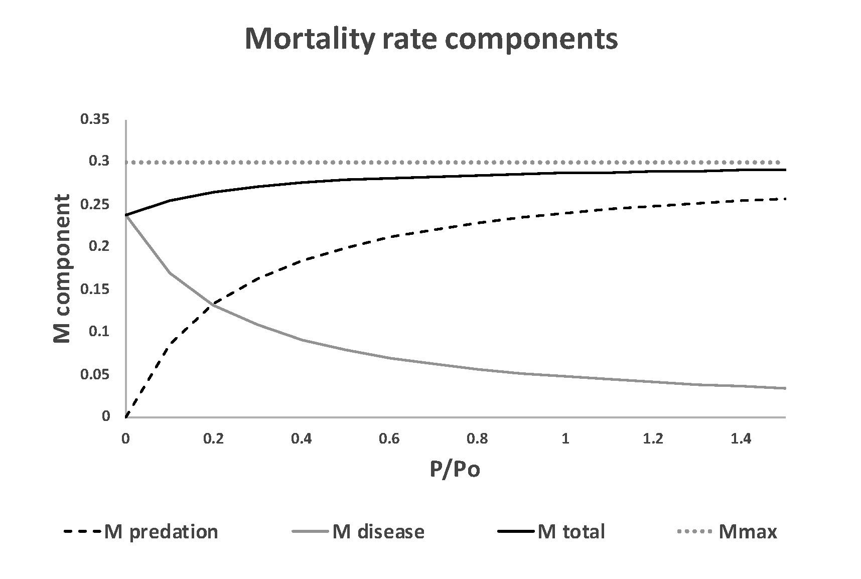
Figure 2. Effect of varying predator biomass P on the total mortality rate M = flow/total biomass B due to predation and stress, for a case where both the instantaneous predation rate paP and stress rate vs are large. In this example, total mortality rate remains close to the vulnerability exchange rate v, even when predator biomass P is zero. See Table 1 for parameter definitions.
If we compare instantaneous mortality rates MP due to predator P for the mass-action and vulnerability exchange formulations as in Figure 2, where MP = (mass eaten per time) / (total prey biomass), we obtain very different predictions about how MP should vary with predator abundance:
Mass-action model:
[latex]M_p=paP\tag{5a}[/latex]
Vulnerability exchange model:
[latex]M_p= \frac {paPV}{B} = \frac {paPv}{v+v'+paP+v_s}\tag{5b}[/latex]
That is, we predict mortality rate to be additive to other mortality rate components and proportional to predator abundance only for cases where the prey are fully vulnerable to predation at all times and are not subject to stress-related mortality, i.e. for cases where v is very large and vs = 0. For the vulnerability exchange case, we predict the total instantaneous mortality rate for the B-P flow link to vary as
[latex]M_{total}=\frac{(paP+v_s) V}{B} = \frac {(paP+v_s ) v}{v+v'+paP+v_s}\tag{6}[/latex]
for which the mortality flow components paPV and vsV are very obviously not additive because of their joint, interacting effect on V.
Predator abundances and forage fish surplus production
To examine how forage fish surplus production rates should vary when Mtotal from Eq. 6 is used to predict the joint effects of predation and stress, suppose we now consider a simple case where there is only a single aggregate predator abundance P and/or all species-size components of the total predation rate are assumed to covary so as to generate a single overall rate that is proportional to the sum of the predator biomass components. Suppose further that we assume the dynamics of B to be dominated by a production-recruitment component that can be adequately described by a Beverton-Holt recruitment function, minus a non-predation mortality rate M0 B minus the total rate MtotalB predicted by Eq. 7, below. Here, M0 is the direct non-predation mortality rate as Mtotal include indirect effects of disease/stress contributions. Under these assumptions, the dynamics of B are given by
[latex]dB⁄dt=(r_{max} B) ⁄ (B_h+B) - (M0+M_{total} B)\tag{7}[/latex]
where rmax is maximum production rate (mass/time), Bh is the forage fish biomass needed to achieve half of this maximum rate, and Mtotal is given for varying P by Eq. 6. Note in Eq. 7 that dB/dt represents the surplus production rate of the forage fish population.
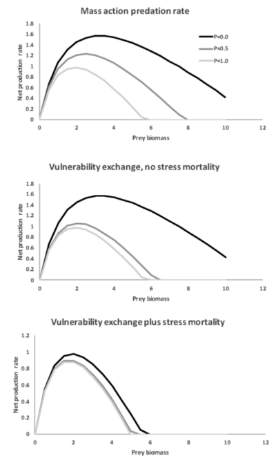
Figure 3. Predicted patterns of variation in the relationship between prey (e.g., forage fish) surplus production rate (dB/dt of Eq. 7) and biomass for different approaches to prediction of predation rates and for varying predator abundances (P, black lines are for high P, light gray for P = 0.0).
Very different patterns of variation in the surplus production vs biomass relationship are predicted by Eq. 7 depending on how predation and stress mortality is represented (Figure 3). For the mass action case (Mtotal = paP) and for vulnerability exchange dynamics without stress factor removal from the vulnerable biomass V, Eq. 7 predicts substantial increase in surplus production when P is reduced. But when Mtotal includes a high mortality rate due to stress when P is low, as in Figure 2, there is almost no response of the predicted surplus production relationship due to reduction in predator abundance.
Note that the patterns predicted in Figure 3 depend importantly on the assumption that foraging time proportion p is stable, i.e. that either there are no handling time effects or that B is a relatively small proportion of the total prey abundance that contributes to predator handling time. When search time does increase substantially at low B, there can be severe depensatory effects that cause reduced or even negative surplus production rates when prey biomass is low.
Simple approximation for non-additive mortality effects
It would be a complex conceptual and programming task to fully represent non-additive mortality patterns like the example in Figure 1 in Ecosim models even for simple stress mortality rate assumptions like vsV with constant vs, because of issues about partitioning Ecopath base unexplained/ other mortality' (M0), and whether to assume different stress-related vulnerability and mortality patterns for each of many predator-prey trophic links in typical Ecosim models. However, the same basic effect as shown in the third panel of Figure 3 can be obtained simply by first calculating the Ecosim predicted predation mortality rate (summed over predator types) at each time step, then adding a component to M0 so as to prevent the total "apparent" predation mortality rate from decreasing to less than a user-defined minimum proportion of the Ecopath base predation mortality rate. This simple convention allows exploration of alternative hypotheses about how much M0 would increase in scenarios where total predator abundance is reduced, using a single parameter (proportion of base predation mortality rate when predation rate is 0.0) to represent "hidden" non-additive (stress factor) effects.
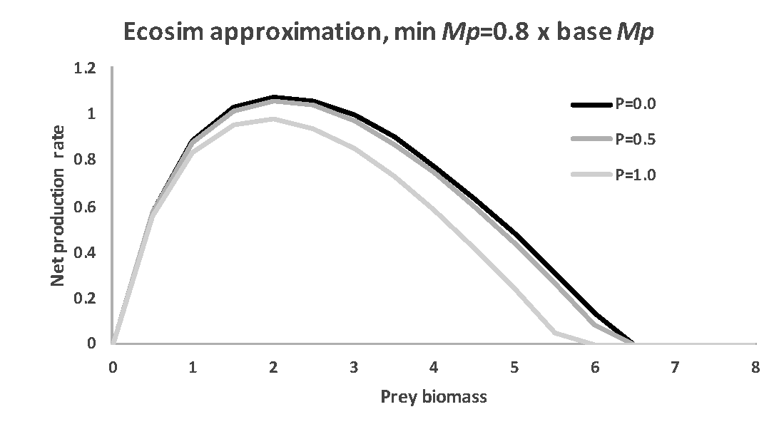
Figure 4. Effect of including a minimum mortality rate component representing non-additive stress mortality on Ecosim predictions of the surplus production vs biomass relationship. Compare this prediction to those in the bottom two panels of Figure 3 – the simple mortality rate constraint causes the Ecosim prediction to be close to that obtained by explicitly modeling non-additive stress mortality.
Effects of such a minimum mortality constraint on the predicted surplus production-biomass relationship for the same parameter values used in Figure 3 is shown in Figure 4. Setting the minimum "hidden" predation rate to 0.8 times the Ecopath base rate causes the predicted surplus production pattern to look almost exactly like the full non-additive mortality pattern in the bottom panel of Figure 3, i.e. to predict very little increase in surplus production when predator abundance is low.
As the ratio of minimum to Ecopath base apparent predation mortality rate is reduced (from 0.8 to lower values for the Figure 4 example), the predicted surplus production pattern shifts to equal the pattern predicted in the middle panel of Figure 3 as the ratio approaches zero.
We caution against using this single-parameter approach just to generate multispecies scenarios where trophic interaction effects are omitted entirely (by setting the additive proportion very low), just to conform with single species modeling theory and experience.
Discussion
It is an old idea in ecology going back at least to Errington[21] that predators may take mainly weak, sick, and old animals, and that it therefore may be perilous to assume that predator control will increase productivity of valuable prey species. In terms of current terminology about top-down (predation) versus bottom-up (prey productivity) control of trophic interactions, low values of the vulnerability exchange rate parameter v in the model presented above imply stronger bottom-up control of predator abundances, while high v values imply at least the possibility of strong top-down control but with the caveat that high vs values may invalidate predictions based just on v and on predator abundance. Our models warn not to expect correct or reliable assessments of relative importance of top-down vs bottom-up effects from correlative studies of abundance variation over time (e.g.[22] [23] [24] because of possible interactive effects of predation and bottom-up "habitat" factors like temperature, as we estimate to be possible for the salmon example.
In evaluation of evidence about the relative importance of top-down effects, we should focus mainly on cases where there have been deliberate manipulations of top-down effects (e.g.,[25] [26] that would reveal existence of vs effects if such effects are indeed present. This warning holds as well for those rare cases where we have direct estimates of variation in natural mortality rates (M) over time from data such as survey relative abundances at age or tagging as in the salmon case; good correlations of M with predator abundance do not imply top-down control when stress factors have changed over time in patterns correlated with predator abundance.
Modern molecular techniques offer considerable promise to screen for gene activation patterns (gene expression profiles) indicative of stress, and hence to directly measure v and V, i.e. whether the prey taken by predators are indeed mainly those that are stressed particularly by diseases (e.g.[27] [28] [29]. But unfortunately, such techniques do not provide direct measures of the virulence of the stress factors, i.e. of the direct stress mortality and recovery rate parameters vs and v’; predation impacts may still be essentially additive components of total M if vs is low.
Another way to examine the credibility of hypotheses about non-additive predation impacts is to compare estimates of predator rates of effective search (a) implied by high vs-low V models with direct estimates of rates of search based on predator characteristics. Such direct estimates can be obtained from basic information on predator movement speeds, reactive distances to prey, and proportions of time spent foraging, combined with information on the effective area or volume over which the search is distributed. For the juvenile salmon-seal example in Walters and Christensen[30], such calculations suggest much lower a parameter values for seals than would be necessary to explain the data under high vs assumptions.
As data sets accumulate with age-specific survey estimates of abundance (from which temporal variation in total natural mortality rate M can be estimated), we will also be able to directly compare observed changes in M with predictions from additive predation models (and direct estimates of search rates). Seeing lower slopes in M vs predator abundance plots than predicted under additive predation would be evidence of high stress-dependent mortality rates (vs), as in the Figure 2 example.
Continued climate change will quite possibility result in substantial changes in trophic interaction patterns[31] through "hidden" effects due to temperature-related changes in v and vs, (e.g., increases in disease expression or physiological impact). But such changes may be "masked" when stressed individuals are rapidly removed by predators, so as to only exert increasing effects when various factors, like fishing, lead to predator abundance declines. This means that climate change is quite likely to produce some very nasty surprises that we will not anticipate through ecosystem models built around simplistic assumptions about additivity of mortality components, nor can we be confident that simpler models based on statistical or correlative historical data will somehow give better predictions.
- Hatcher, M.J., Dick, J.T., Dunn, A.M., 2012. Diverse effects of parasites in ecosystems: linking interdependent processes. Frontiers in Ecology and the Environment 10, 186–194. https://doi.org/10.1890/110016 ↵
- Krkošek, M., 2017. Population biology of infectious diseases shared by wild and farmed fish1. Can J Fish Aquat Sci 74, 620–628. https://doi.org/10.1139/cjfas-2016-0379 ↵
- Sures, B., Nachev, M., Pahl, M., Grabner, D., Selbach, C., 2017. Parasites as drivers of key processes in aquatic ecosystems: Facts and future directions. Exp. Parasitol. 180, 141–147. https://doi.org/10.1016/j.exppara.2017.03.011 ↵
- Gray, R., Fulton, E., Little, R., Scott, R., 2006. Ecosystem model specification with an agent based framework. Technical report CSIRO. Marine and Atmospheric Research. North West Shelf Joint Environmental Management Study; no. 1–139. ↵
- Engelhard, G.H., Peck, M.A., Rindorf, A., C Smout, S., van Deurs, M., Raab, K., Andersen, K.H., Garthe, S., Lauerburg, R.A.M., Scott, F., Brunel, T., Aarts, G., van Kooten, T., Dickey-Collas, M., 2014. Forage fish, their fisheries, and their predators: who drives whom? ICES JMS 71, 90–104. https://doi.org/10.1093/icesjms/fst087 ↵
- Koehn, L.E., Essington, T.E., Marshall, K.N., Kaplan, I.C., Sydeman, W.J., Szoboszlai, A.I., Thayer, J.A., 2016. Developing a high taxonomic resolution food web model to assess the functional role of forage fish in the California Current ecosystem. Ecol Model 335, 87–100. https://doi.org/10.1016/j.ecolmodel.2016.05.010 ↵
- Walters, C.J., Christensen, V., Martell, S.J., Kitchell, J.F., 2005. Possible ecosystem impacts of applying MSY policies from single-species assessment. ICES JMS 62, 558–568. https://doi.org/10.1016/j.icesjms.2004.12.005 ↵
- Szuwalski, C.S., Burgess, M.G., Costello, C., Gaines, S.D., 2017. High fishery catches through trophic cascades in China. Proc. Natl. Acad. Sci. U.S.A. 114, 717–721. https://doi.org/10.1073/pnas.1612722114 ↵
- Walters, C., Christensen, V., Pauly, D., 1997. Structuring dynamic models of exploited ecosystems from trophic mass-balance assessments. Rev Fish Biol Fisheries 7, 139–172. https://doi.org/10.1023%2fa%3a1018479526149 ↵
- Scott, F., Blanchard, J.L., Andersen, K.H., 2014. mizer: an R package for multispecies, trait-based and community size spectrum ecological modelling. Methods in Ecology and Evolution 5, 1121–1125. https://doi.org/10.1111/2041-210X.12256 ↵
- Jacobsen, N.S., Essington, T.E., Andersen, K.H., 2015. Comparing model predictions for ecosystem-based management1. Can J Fish Aquat Sci 73, 666–676. https://doi.org/10.1139/cjfas-2014-0561 ↵
- Jacobsen, N.S., Thorson, J.T., Essington, T.E., 2019. Detecting mortality variation to enhance forage fish population assessments. ICES JMS 76, 124–135. https://doi.org/10.1093/icesjms/fsy160 ↵
- Garcia, S.M., J Kolding, J Rice, Rochet, M.-J., Zhou, S., Arimoto, T., Beyer, J.E., Borges, L., Bundy, A., Dunn, D., Fulton, E.A., Hall, M., M Heino, Law, R., M Makino, Rijnsdorp, A.D., Simard, F., Smith, A.D.M., 2012. Reconsidering the consequences of selective fisheries. Science 335, 1045–1047. http://dx.doi.org/10.1126/science.1214594 ↵
- Walters et al. 1997, https://doi.org/10.1016/j.ecolmodel.2019.108776 op. cit. ↵
- Ahrens, R.N.M., Walters, C.J., Christensen, V., 2012. Foraging arena theory. Fish Fish. 13, 41–59. https://doi.org/10.1111/j.1467-2979.2011.00432.x ↵
- Walters C, Christensen V. 2019. Effect of non-additivity in mortality rates on predictions of potential yield of forage fishes. Ecological Modelling, 410: #108776. https://doi.org/10.1016/j.ecolmodel.2019.108776 ↵
- Essington, T.E., Munch, S.B., 2014. Trade‐offs between supportive and provisioning ecosystem services of forage species in marine food webs. Ecol Model 24, 1543–1557. https://doi.org/10.1890/13-1403.1 ↵
- Holling, C.S., 1959. The components of predation as revealed by a study of small mammal predation of the European pine sawfly 91, 293–320. https://doi.org/10.4039/Ent91293-5 ↵
- Walters et al., 1997. https://doi.org/10.1016/j.ecolmodel.2019.108776 op. cit. ↵
- Walters, C.J., Juanes, F., 1993. Recruitment limitation as a consequence of natural selection for use of restricted feeding habitats and predation risk taking by juvenile fishes. Can J Fish Aquat Sci 50, 2058–2070. https://doi.org/10.1139/f93-22 ↵
- Errington, P.L., 1946. Predation and Vertebrate Populations (Concluded). The Quarterly Review of Biology 21, 221–245. https://doi.org/10.1086/395315 ↵
- Boyce, D.G., Frank, K.T., Worm, B., Leggett, W.C., 2015. Spatial patterns and predictors of trophic control in marine ecosystems. Ecol Lett 18, 1001–1011. https://doi.org/10.1111/ele.12481 ↵
- Lynam, C.P., Llope, M., Möllmann, C., Helaouët, P., Bayliss-Brown, G.A., Stenseth, N.C., 2017. Interaction between top-down and bottom-up control in marine food webs. Proc. Natl. Acad. Sci. U.S.A. 114, 1952–1957. https://doi.org/10.1073/pnas.1621037114 ↵
- Ye, Y., Carocci, F., 2019. Control mechanisms and ecosystem‐based management of fishery production. Fish and Fisheries 20, 15–24. https://doi.org/10.1111/faf.12321 ↵
- Borer, E.T., Halpern, B.S., Seabloom, E.W., 2006. Asymmetry in community regulation: effects of predators and productivity. Ecology 87, 2813–2820. https://doi.org/10.1890/0012-9658(2006)87[2813:aicreo]2.0.co;2 ↵
- McClanahan, T.R., Muthiga, N.A., Coleman, R.A., 2011. Testing for top‐down control: can post‐disturbance fisheries closures reverse algal dominance? Aquatic Conservation: Marine and Freshwater Ecosystems 21, 658–675. https://doi.org/10.1002/aqc.1225 ↵
- Jeffries, K.M., Hinch, S.G., Gale, M.K., Clark, T.D., Lotto, A.G., Casselman, M.T., Li, S., Rechisky, E.L., Porter, A.D., Welch, D.W., Miller, K.M., 2014. Immune response genes and pathogen presence predict migration survival in wild salmon smolts. Mol Ecol 23, 5803–5815. https://doi.org/10.1111/mec.12980 ↵
- Miller, K.M., Teffer, A., Tucker, S., Li, S., Schulze, A.D., Trudel, M., Juanes, F., Tabata, A., Kaukinen, K.H., Ginther, N.G., Ming, T.J., Cooke, S.J., Hipfner, J.M., Patterson, D.A., Hinch, S.G., 2014. Infectious disease, shifting climates, and opportunistic predators: cumulative factors potentially impacting wild salmon declines. Evol Appl 7, 812–855. https://doi.org/10.1111/eva.12164 ↵
- Tucker, S., Li, S., Kaukinen, K.H., Patterson, D.A., Miller, K.M., 2018. Distinct seasonal infectious agent profiles in life-history variants of juvenile Fraser River Chinook salmon: An application of high-throughput genomic screening. PLoS ONE 13, e0195472. https://doi.org/10.1371/journal.pone.0195472 ↵
- Walters and Christensen. 2019. https://doi.org/10.1016/j.ecolmodel.2019.108776 op. cit. ↵
- Lynam et al., 2017. https://doi.org/10.1073/pnas.1621037114 op. cit. ↵
- Walters and Christensen, 2019, https://doi.org/10.1016/j.ecolmodel.2019.108776 op. cit. ↵
